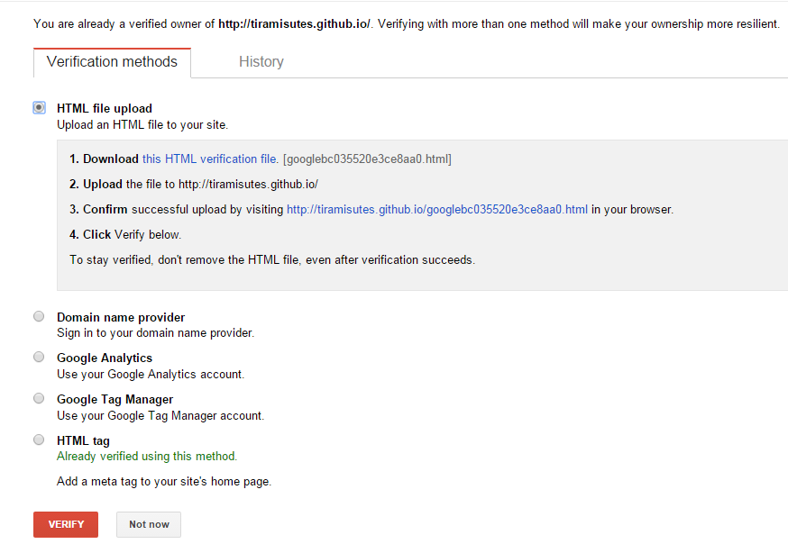
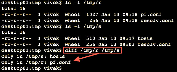
hopeA new day is coming,whether we like it or not. The question is will you control it,or will it control you?2021-10-21T14:02:23.577Zhttp://tiramisutes.github.io/tiramisutes1099808298@qq.comHexo植物单细胞转录组数据库PsctHhttp://tiramisutes.github.io/2021/10/21/PsctH.html2021-10-21T13:55:09.000Z2021-10-21T14:02:23.577Z作为所有生物体的基本组成部分,细胞在维持生命活动中起着至关重要的作用,而作为细胞异质性研究的重要工具,近年来单细胞转录组测序技术蓬勃发展,促使生物学研究进入单细胞水平的时代。然而,在植物学领域,单细胞的研究仍处于起步阶段,可用资源非常有限,且单细胞悬浮液(即原生质悬浮液)的制备和细胞簇的注释仍然是阻碍其研究的两大主要障碍。 近日,知名期刊Plant Biotechnology Journal在线发表了华中农业大学棉花遗传改良团队金双侠教授团队的篇题为《Plant Single Cell Transcriptome Hub (PsctH): an integrated online tool to explore the plant single-cell transcriptome landscape》论文,开发了植物单细胞转录组综合数据库PsctH,提供综合全面的单细胞Marker基因资源和单细胞研究的workflow。 PsctH主要包括植物单细胞悬浮液的制备手册,植物单细胞转录组分析流程的个性化定制,植物单细胞Marker基因资源和植物单细胞测序原始数据集四大板块,综合了单细胞研究的整个过程。 不同于动物细胞,细胞壁的存在使得植物单细胞悬浮液的制备更加困难。根据实验室前期原生质体解离实验经验,作者比较和评估了用于制备原生质体的不同方案,并提供了一套可行和高效的植物单细胞悬浮液制备手册,其中包括组织样品的制备和分离、酶解消化、纯化以及单个细胞完整性检测。同时,还提供了灵活的植物单细胞转录组(scRNA-seq)分析流程,包括质量控制、标准化、聚类和标记基因鉴定过程。同时考虑到单细胞研究的复杂性和大数据量,暂时并未提供相应的在线分析,而是通过配置关键参数以获得特定的R语言分析脚本。此外,还提供了配置数据分析的R环境文件(SingleCellCondaEnvironment.yml),研究人员可以通过conda再现单细胞转录组的分析环境,来运行之前获得的R脚本。 另一方面,由于缺乏有效的Marker基因资源,植物单细胞研究通常需要花费大量的时间来进行RNA原位杂交或报告基因的遗传转化来为细胞簇的组织类型鉴定提供可靠的实验证据。因此,作者通过收集目前植物单细胞研究,获取到来自5种植物(拟南芥、玉米、水稻、花生和番茄)的9个组织或亚组织的51种细胞类型的共计98个Marker基因(均经过RNA原位杂交或报告基因验证),并在PsctH的MarkerGeneDB栏目进行保存和展示。 此外,PsctH还提供目前植物单细胞测序原始数据集,植物单细胞文献的挖掘等功能。伴随单细胞研究的快速发展,数据库也采用定期跟新(包括新的功能和现有数据库内容,特别是Marker基因资源)的原则,也欢迎该领域研究人员提供相关资源和建议。
]]>
<p>作为所有生物体的基本组成部分,细胞在维持生命活动中起着至关重要的作用,而作为细胞异质性研究的重要工具,近年来单细胞转录组测序技术蓬勃发展,促使生物学研究进入单细胞水平的时代。然而,在植物学领域,单细胞的研究仍处于起步阶段,可用资源非常有限,且单细胞悬浮液(即原生质悬浮液)的制备和细胞簇的注释仍然是阻碍其研究的两大主要障碍。<br>近日,知名期刊Plant Biotechnology Journal在线发表了华中农业大学棉花遗传改良团队金双侠教授团队的篇题为《<a href="https://onlinelibrary.wiley.com/doi/10.1111/pbi.13725" target="_blank" rel="noopener">Plant Single Cell Transcriptome Hub (PsctH): an integrated online tool to explore the plant single-cell transcriptome landscape</a>》论文,开发了植物单细胞转录组综合数据库<a href="http://jinlab.hzau.edu.cn/PsctH/" target="_blank" rel="noopener">PsctH</a>,提供综合全面的单细胞Marker基因资源和单细胞研究的workflow。<br>
Nature Methods | 多伦多大学通过优化KRAB来提高CRISPRi对靶基因的沉默效果http://tiramisutes.github.io/2020/10/07/CRISPRi.html2020-10-07T06:16:32.000Z2020-10-07T06:32:05.430ZCRISPRi 简介
此外,在dCas9-KRAB融合蛋白前加一个条件性启动子可进行条件性CRISPRi。将若干sgRNA、启动子和dCas9-KRAB串联表达可同时进行多重基因的CRISPRi,实现多基因的同时沉默等优势(Zheng, Y., Shen, W., Zhang, J. et al. CRISPR interference-based specific and efficient gene inactivation in the brain. Nat Neurosci 21, 447–454 (2018). https://doi.org/10.1038/s41593-018-0077-5 )。
CRISPRi与CRISPR区别
尽管CRISPR相关工具的基因敲除在基因功能研究和性状改良方面有重要的应用,但同时也存在其局限性。如某个基因功能的完全丧失会产生极端表型,而育种过程中通常想要的是中间表型。此外,CRISPRi可靶向lncRNA、microRNA、反向转录产物、细胞核内的转录本等,是研究非蛋白编码基因的有力工具(图2)。 尽管CRISPRi如此优秀,但目前也存在一些“小问题”,如靶基因的不完全沉默;PAM序列在一定程度上限制了结合靶序列的数量;染色体状态和修饰可能会影响dCas9-gRNA与DNA的结合;当靶基因的靶序列与其它基因重叠,或受双向启动子调节时,CRISPRi的调控可能会影响到周边的基因表达。 图2. 功能缺失或功能获得系统示意图。(ACS Chem Biol. 2018 Feb 16;13(2):406-416)
CRISPRi优化
近日,知名植物学期刊Nature Methods在线发表了多伦多大学和加拿大高等研究院(CIFAR)题为An efficient KRAB domain for CRISPRi applications in human cells的研究论文。通过优化KRAB domain来提高对靶基因的沉默效果,并筛选出目前基因沉默效果最具高效的ZIM3 KRAB–dCas9载体。 作者将57个人的KRAB结构域融合到dCas9的N端,并用慢病毒感染法检测它们被招募到两个不同的含报告基因结构中时的活性。其中一种方法是将dCas9-KRAB融合靶向到SV40启动子上的两个位点,该启动子驱动人类胚胎肾器官293T细胞(HEK293T)中绿色荧光蛋白(EGFP)的表达。在另一组实验中,dCas9-KRAB融合蛋白靶向K562细胞的PGK1-EGFP报告基因下游的7×TetO阵列上(图3)。且两种报告细胞系均来自单细胞克隆,以确保报告基因和gRNA表达水平的一致性。 图3. KRAB结构域筛选系统。
2004 A CDC45 Homolog in Arabidopsis Is Essential for Meiosis, as Shown by RNA Interference–Induced Gene Silencing 如RNA干扰诱导的基因沉默所示,拟南芥CDC45同系物对减数分裂至关重要 http://www.plantcell.org/content/16/1/99 2007 A CLASSY RNA Silencing Signaling Mutant in Arabidopsis 拟南芥一个RNA沉默信号突变株 http://www.plantcell.org/content/19/5/1439 2007 A CRM Domain Protein Functions Dually in Group I and Group II Intron Splicing in Land Plant Chloroplasts 陆地植物叶绿体中CRM结构域蛋白在Ⅰ组和Ⅱ组内含子剪接中的双重功能 http://www.plantcell.org/content/19/12/3864 2015 A Cascade of Sequentially Expressed Sucrose Transporters in the Seed Coat and Endosperm Provides Nutrition for the Arabidopsis Embryo 种皮和胚乳中蔗糖转运蛋白的级联表达为拟南芥胚胎提供了营养 http://www.plantcell.org/content/27/3/607 2011 A Case for Spatial Regulation in Tetrapyrrole Biosynthesis 四吡咯生物合成的空间调控 http://www.plantcell.org/content/23/12/4167 2001 A Cell Plate–Specific Callose Synthase and Its Interaction with Phragmoplastin 细胞板特异性胼胝质合成酶及其与胞浆蛋白的相互作用 http://www.plantcell.org/content/13/4/755 2009 A Cell Wall–Degrading Esterase of Xanthomonas oryzae Requires a Unique Substrate Recognition Module for Pathogenesis on Rice 水稻黄单胞菌的细胞壁降解酯酶需要一个独特的底物识别模块来研究水稻的发病机制 http://www.plantcell.org/content/21/6/1860
2019年10月16日,国际学术期刊Nature Communications在线发表了中国热带农业科学院香料饮料研究所联合华中农业大学、马来西亚科学院等7家单位完成的题为“The chromosome-scale reference genome of black pepper provides insight into piperine biosynthesis”的研究论文。该研究绘制了我国胡椒栽培种“热引1号”染色体级别精细基因组图谱(木兰亚纲胡椒目首次报道基因组组装的物种),综合解读胡椒的基因组特征,物种进化位置,并进一步对胡椒碱合成代谢网络和关键基因及其基因家族进行深入研究,为被子植物演化及胡椒碱生物合成提供了新的见解。
C.H. and S.J. designed and supervised the research. Z.X. performed the genome assemblies and annotation. Z.X. and L.H. performed the transcriptome and phylogenetic analysis. L.H., H.W., X.Q., L.Y. and L.T. collected materials for sequencing and generated transcriptome data. Z.X., L.H., R.F. and B.W. analysed the RNA-seq data. M.W., D.Y., S.S., W.L., C.S., H.D., J.W., K.L. and X.Z. provided constructive comments and suggestions on data analysis. Z.X. and L.H. wrote the paper with input from all other authors. All authors approved the paper.
The chromosome-scale reference genome of black pepper provides insight into piperine biosynthesis 类型 期刊文章 作者 Lisong Hu 作者 Zhongping Xu 作者 Maojun Wang 作者 Rui Fan 作者 Daojun Yuan 作者 Baoduo Wu 作者 Huasong Wu 作者 Xiaowei Qin 作者 Lin Yan 作者 Lehe Tan 作者 Soonliang Sim 作者 Wen Li 作者 Christopher A. Saski 作者 Henry Daniell 作者 Jonathan F. Wendel 作者 Keith Lindsey 作者 Xianlong Zhang 作者 Chaoyun Hao 作者 Shuangxia Jin URL https://www.nature.com/articles/s41467-019-12607-6 版权 2019 The Author(s) 卷 10 期 1 页码 1-11 期刊 Nature Communications ISSN 2041-1723 日期 2019-10-16 刊名缩写 Nat Commun DOI 10.1038/s41467-019-12607-6 访问时间 10/23/2019, 11:55:31 AM 馆藏目录 www.nature.com 语言 en 摘要 Black pepper (Piper nigrum) belongs to the long-isolated lineage of basal angiosperm and its fruit has been used for food spice and phytomedicines for thousands of years. Here, the authors assemble the reference genome of this species and analyze gene families associated with piperine biosynthesis. 添加日期 10/23/2019, 11:55:31 AM 修改日期 10/23/2019, 11:55:31 AM
目前,主要通过化学杀虫剂对苹果蠹蛾进行管控,但已出现明显抗性。了解其抗药性机制对于进一步的害虫防御起到重要的作用。苹果蠹蛾主要的抗药性机制依赖于解毒酶活性的提高和降低靶蛋白对杀虫剂的敏感性。作者在苹果蠹蛾中共鉴定到667个潜在杀虫剂抗性相关基因,包括434个解毒基因,45个杀虫剂目标基因,124个角质层基因,47个ABC转运蛋白和12个水通道蛋白。之前的研究表明P450基因赋予苹果蠹蛾对杀虫剂的光谱抗性。因此,作者对苹果蠹蛾基因组中的P450基因进行深入研究。 146个P450基因在基因组的染色体分布显示有16个基因簇包含3个或更多的P450基因。其中位于chr20染色体的基因簇包含11个基因,包括3个CYP6AE基因。 为确定P450基因数目的增加赋予苹果蠹蛾对杀虫剂的抗虫,作者对来自三个种群的(S, Raz和Rv)苹果蠹蛾各随机挑选6个个体进行40X的重测序,S种群对杀虫剂敏感,自1995年起没有暴露在任何杀虫剂中;Raz种群对杀虫剂有抗性,自1997年起幼虫暴露在甲基谷硫磷中,相较于S种群表现出对甲基谷硫磷7倍的抗性,对西维因130倍的抗性;RV种群自1995年起幼虫暴露于溴氰菊酯,相较于S种群,表现出对溴氰菊酯140倍的抗性。 GWAS分析在S 和 Raz种群中共鉴定到109个具显著不同的等位基因频率的SNPs位于上述667个耐药相关基因的外显子区。S 和 Rv种群的比较共鉴定到242个具显著差异的SNPs位于耐药相关基因的外显子区,其中18个SNPs是Raz 和Rv种群共有的。对于其中的11个SNPs对,选取每个种群的数十个个体通过Sanger测序进行进一步的分析,确认了其中7个SNPs在S与Raz或Rv种群间存在固定的差异。验证的SNPs在毒蕈碱受体(mAChR),章鱼胺β受体和P450基因CYP6B2中的突变因相关基因从未报道参与到鳞翅目昆虫的杀虫剂抗性中而引起作者的注意。 随后作者对苹果蠹蛾的P450基因通过RACE进行5’UTR的注释,结果136个P450基因有69个完成5’UTR的注释 ,并将这69个P450基因比对到基因组scaffolds进行转录起始位点和启动子的注释。136个P450基因中,GWAS分析分别鉴定到128和203个SNPs在S种群和Raz或Rv种群间存在差异。在69个基因的启动子区中,分别鉴定到9和10个SNPs在S种群和Raz或Rv种群间存在差异。特别的,有3个SNPs均存在于Raz和Rv种群的CYP6B2基因启动子区:A52T: A (−52)T,T(−57)T,和T(−110)G (gene ID: CPOM05212)。qPCR对三个种群中的CYP6B2基因的表达进行测定,结果表明该基因相较于S种群,在两个抗性种群中(241.4-fold in Raz and 77.3-fold in Rv)组成性高表达,表明这3个SNPs在CYP6B2基因的表达调控中起到重要作用。 进一步为确认CYP6B2基因的表达与杀虫剂抗性相关,作者对来自酒泉的四龄测序苹果蠹蛾通过siRNA注射敲除CYP6B2基因,结果48小时后CYP6B2基因的表达下降55%,并用LC50浓度的甲基谷硫磷,溴氰菊酯和吡虫啉饲喂RNAi个体。结果饲喂甲基谷硫磷和溴氰菊酯的幼虫成活率分别为31.1%和45.6%,显著低于GFP注射的对照组或不做任何处理的分组,表明敲除CYP6B2基因显著增加对甲基谷硫磷和溴氰菊酯的敏感性,而幼虫对吡虫啉的敏感性并未受影响。综合表明CYP6B2基因赋予苹果蠹蛾对两个广泛使用的杀虫剂的抗性中起到关键作用。
map1 <- cnmapdf %>% filter(prov_en %in% unique(cnmapdf$prov_en)) %>% ggplot() + geom_polygon(aes(x = long, y = lat, group = group, fill = prov_cn), color = "grey")
R Visual. - China Map Part II https://www.datanovia.com/en/blog/ggplot-colors-best-tricks-you-will-love/ https://www.datanovia.com/en/blog/top-r-color-palettes-to-know-for-great-data-visualization/ 标准中国地图的绘制
]]>
<p>在重测序文章中经常见到用地图来描述测序样品分布,而地图涉及到主权,属敏感问题,但在R中可轻(fu)松(za)复现。<br><img src="/images/map0.png" alt=""><br>
分子生物学 or 生物信息学, that's a questionhttp://tiramisutes.github.io/2019/04/18/Biotechnology-Vs-Bioinformatics.html2019-04-18T05:40:50.000Z2019-04-19T15:50:42.566Z 分子生物学(Molecular biology)是对生物在分子层次上的研究,是生物学和化学之间跨学科的研究,其研究领域涵盖了遗传学、生物化学和生物物理学等学科。分子生物学主要致力于对细胞中不同系统之间相互作用的理解,包括DNA,RNA和蛋白质生物合成之间的关系以及了解它们之间的相互作用是如何被调控的。 在我们的研究中主要涉及基因功能和代谢通路解析; 生物信息学(Bioinformatics)利用应用数学、信息学、统计学和计算机科学的方法研究生物学的问题。生物信息学的研究材料和结果就是各种各样的生物学数据,其研究工具是计算机,研究方法包括对生物学数据的搜索(收集和筛选)、处理(编辑、整理、管理和显示)及利用(计算、模拟)。当前主要的研究方向有:序列比对、序列组装、基因识别、基因重组、蛋白质结构预测、基因表达、蛋白质反应的预测,以及创建进化模型。 自迈克尔·沃特曼(Michael Waterman)率先将数学和计算方法引入生物学研究开始,如今这门交叉学科作为后起之秀正逐渐渗透到生物学研究的多个领域,21世纪是生命科学的世纪,但也是一个信息化的时代,如果做分子的不懂生信,做生信的不懂分子,如何让自己走的更远? 工欲善其事,必先利其器,各行各业都有其不二法宝,科研工作亦当如此;
template.sbt (this is the only file whose prefix is different. Leave the prefix as is). chr01.fsa chr01.tbl chr01.qvl
4.1 特殊参数解释
-i 指定fa文件名,且一定不能包含路径,只能是文件名;
-M 参数会覆盖部分其他参数;
-l 只有当 -M 设置为 t 时才可用;
-a s: fa文件包含多个序列,结果生成单个提交文件;
4.2 运行实例
1
2
cd NCBI_Genome linux64.tbl2asn -p . -r . -t template.sbt -i genome.fa -a s -j "[organism=xx][genotype=xx][tech=wgs][country=China]" -V vbgt -k c -Z discrep.txt -N 1.0 -L T -n xx
#!/usr/bin/env python """Convert a GFF and associated FASTA file into GenBank format. Usage: gff_convert.py -f genbank -s <GFF annotation file> <FASTA sequence file> """ import sys import os from Bio import SeqIO from Bio.Alphabet import generic_dna from Bio import Seq import argparse from BCBio import GFF
parser=argparse.ArgumentParser( description='''Script that converts GFF + Fasta to GBK or EMBL ''', epilog="""hope (2019) http://tiramisutes.github.io/2019/04/05/PBGNCBI.html""") parser.add_argument("gff", help='GFF file') parser.add_argument("fasta", help='Fasta file') parser.add_argument("-f", "--format", choices=['genbank', 'embl']) parser.add_argument("-s","--split", action='store_true', help='Split output into single files, 1 per contig') parser.add_argument("-o","--output", help='Set the directory of output file/files') args=parser.parse_args()
if len(sys.argv) < 2: parser.print_usage() sys.exit(1)
def_fix_ncbi_id(fasta_iter): """GenBank identifiers can only be 16 characters; try to shorten NCBI. """ for rec in fasta_iter: if len(rec.name) > 16and rec.name.find("|") > 0: new_id = [x for x in rec.name.split("|") if x][-1] print"Warning: shortening NCBI name %s to %s" % (rec.id, new_id) rec.id = new_id rec.name = new_id yield rec
def_check_gff(gff_iterator): """Check GFF files before feeding to SeqIO to be sure they have sequences. """ for rec in gff_iterator: if isinstance(rec.seq, Seq.UnknownSeq): print"Warning: FASTA sequence not found for '%s' in GFF file" % ( rec.id) rec.seq.alphabet = generic_dna yield _flatten_features(rec)
def_flatten_features(rec): """Make sub_features in an input rec flat for output. GenBank does not handle nested features, so we want to make everything top level. """ out = [] for f in rec.features: cur = [f] while len(cur) > 0: nextf = [] for curf in cur: out.append(curf) if len(curf.sub_features) > 0: nextf.extend(curf.sub_features) cur = nextf rec.features = out return rec
if args.split: if format == "genbank": print("Output set to " + format + ", splitting files and writting individual records to directory: " + output_dir) fasta_input = SeqIO.to_dict(SeqIO.parse(fasta_file, "fasta", generic_dna)) for rec in GFF.parse(gff_file, fasta_input): SeqIO.write(_check_gff(_fix_ncbi_id([rec])), open(output_dir + "/" + rec.id + ".gbk", "w"), "genbank") if format == "embl": print("Output set to " + format + ", splitting files and writting individual records to directory: " + output_dir) fasta_input = SeqIO.to_dict(SeqIO.parse(fasta_file, "fasta", generic_dna)) for rec in GFF.parse(gff_file, fasta_input): SeqIO.write(_check_gff(_fix_ncbi_id([rec])), open(output_dir + "/" + rec.id + ".embl", "w"), "embl") else: if format == "genbank": out_file = output_dir + "/%s.gb" % os.path.splitext(os.path.basename(gff_file))[0] print("Output set to " + format + ", writing file to " + out_file) fasta_input = SeqIO.to_dict(SeqIO.parse(fasta_file, "fasta", generic_dna)) gff_iter = GFF.parse(gff_file, fasta_input) SeqIO.write(_check_gff(_fix_ncbi_id(gff_iter)), out_file, "genbank") if format == "embl": out_file = output_dir + "/%s.embl" % os.path.splitext(os.path.basename(gff_file))[0] print("Output set to " + format + ", writing file to " + out_file) fasta_input = SeqIO.to_dict(SeqIO.parse(fasta_file, "fasta", generic_dna)) gff_iter = GFF.parse(gff_file, fasta_input) SeqIO.write(_check_gff(_fix_ncbi_id(gff_iter)), out_file, "embl")
]]>
<p><img src="/images/sra.png" alt=""><br>
Nature Communications | 苹果为什么那么红http://tiramisutes.github.io/2019/04/03/apple.html2019-04-03T05:14:26.000Z2019-04-03T13:39:19.126Z 研究表明,苹果的祖先原是灌木,大约6000万年前地球遭遇巨型陨石袭击时,大量灰尘被推入大气层中,遮蔽了阳光,降低了植物的光合作用,进而对全球各地的生态系统造成毁灭性的影响,令地球上的大部分生物包括恐龙灭绝,而苹果的祖先却死里逃生,通过进化获得了新生。 苹果、葡萄、柑桔和香蕉并称为世界四大水果,而苹果更是四大水果之冠。“一天一个苹果”是人们熟知的健康口号。自19世纪起威尔士就有俗语说明苹果和健康的关系:“一天一苹果,医生远离我”(An apple a day keeps the doctor away)。 的确,苹果含有丰富的糖类、有机酸、纤维素、维生素、矿物质、多酚及黄酮类营养物质,被科学家称为“全方位的健康水果”。依照美国农业部的数据,一份约重242克的苹果热量为126卡,含有大量的膳食纤维及维他命C。苹果皮中含有许多不确定营养价值的植物化学成分,在体外实验中可能有抗氧化作用。苹果中含有槲皮素、儿茶素及原花色素B2等酚类物质。【维基百科:苹果】 同时苹果也是蔷薇科中种类最多和最具经济效益的水果,所以不仅在生活中受人们喜欢,在科学研究中也备受青睐。 苹果基因组对于遗传研究和育种(抗寒,口味,成熟期等)具有重要的意义,同样高质量的染色体级参考基因组(High quality chromosome-scale reference genome)能够更加真实的反应物种基因组信息;截至目前为止(2019年4月),共有4篇高水平文章报道了苹果基因组研究情况。 基因组研究揭示苹果其实是接受了部分“西方价值观”的亚洲移民【果壳 | 苹果:饱含历史又饱受沧桑】。2017年国际著名学术期刊 Nature Communications 更是以 《Genome re-sequencing reveals the history of apple and supports a two-stage model for fruit enlargement》为题在分子水平上揭示了苹果起源、演化和驯化的规律,并证明世界栽培苹果起源于我国新疆。 苹果基因组中首先被测序的是二倍体品种金冠苹果(Golden Delicious),在2017年 Nature Genetics 文章中其基因组Scaffolds N50已达到5.558Mb,属高质量参考基因组水平,通过基因组信息揭示了发生于21MYA前的转座子(transposable elements)爆炸式扩增与天山山脉(苹果的起源中心)的隆起时期相吻合,表明 TEs 在苹果祖先种的多样化和与梨的分歧中起到重要的作用; 2019年4月2日,国际著名学术期刊 Nature Communications 以 《A high-quality apple genome assembly reveals the association of a retrotransposon and red fruit colour》 为题发表了来自中国农科院(辽宁)等单位联合的苹果基因组最新成果,在基因组水平揭示了苹果为什么那么红的原因。 既然已经有高质量参考基因组那么还有必要再测一个吗?当然有,如同人类基因组计划和精准医疗,金冠苹果(Golden Delicious)是美国主栽品种,而中国苹果常栽品种可分为:元帅系,金冠系和富士系,且中国苹果现在栽种面积最大的是富士系苹果,以红富士为主要的栽种品种 (苹果种类及中国苹果常栽品种):
]]>
<p><img src="/images/RedApple.jpg" alt=""><br> 研究表明,苹果的祖先原是灌木,大约6000万年前地球遭遇巨型陨石袭击时,大量灰尘被推入大气层中,遮蔽了阳光,降低了植物的光合作用,进而对全球各地的生态系统造成毁灭性的影响,令地球上的大部分生物包括恐龙灭绝,而苹果的祖先却死里逃生,通过进化获得了新生。<br> 苹果、葡萄、柑桔和香蕉并称为世界四大水果,而苹果更是四大水果之冠。“一天一个苹果”是人们熟知的健康口号。自19世纪起威尔士就有俗语说明苹果和健康的关系:“一天一苹果,医生远离我”(An apple a day keeps the doctor away)。<br> 的确,苹果含有丰富的糖类、有机酸、纤维素、维生素、矿物质、多酚及黄酮类营养物质,被科学家称为“全方位的健康水果”。依照美国农业部的数据,一份约重242克的苹果热量为126卡,含有大量的膳食纤维及维他命C。苹果皮中含有许多不确定营养价值的植物化学成分,在体外实验中可能有抗氧化作用。苹果中含有槲皮素、儿茶素及原花色素B2等酚类物质。【维基百科:苹果】<br>
纳米孔测序系列之基础介绍http://tiramisutes.github.io/2019/03/12/Oxford-Nanopore.html2019-03-12T13:39:59.000Z2019-03-12T15:21:03.081Z纳米孔测序技术
基因组: 目前测序平均reads长度在20Kb以上,最长reads的N50高达48kKb左右,而最长reads可达到惊人的1.29M; 转录组: raw data数据量在2.5~4.4Gb,reads数为2.8~3.9M,其中N50在1.5kb左右,平均长度为1.0kb,平均质量值Q7以上。在对其进行质控后,其基因组比对率在85%左右。
#!/bin/bash for fn in data/DRR0161{25..40}; do samp=`basename ${fn}` echo"Processing sample ${samp}" salmon quant -i athal_index -l A \ -1 ${fn}/${samp}_1.fastq.gz \ -2 ${fn}/${samp}_2.fastq.gz \ -p 8 -o quants/${samp}_quant done
后续差异基因分析
Once you have your quantification results you can use them for downstream analysis with differential expression tools like DESeq2, edgeR, limma, or sleuth. Using the tximport package, you can import salmon’s transcript-level quantifications and optionally aggregate them to the gene level for gene-level differential expression analysis. You can read more about how to import salmon’s results into DESeq2 by reading the tximport section of the excellent DESeq2 vignette. For instructions on importing for use with edgeR or limma, see the tximport vignette. For preparing salmon output for use with sleuth, see the wasabi package.
==首选 DESeq 的方法;==
一、Analysing no replicate RNA-seq data with LPEseq package
LPEseq was designed for the RNA-Seq data with a small number of replicates, especially with non-replicate in each class. Also LPEseq can be equally applied both count-base and FPKM-based (non-count values) input data.
二、IsoEM2
三、edgeR
The quasi-likelihood method is highly recommended for differential expression analyses of bulk RNA-seq data as it gives stricter error rate control by accounting for the uncertainty in dispersion estimation. The likelihood ratio test can be useful in some special cases such as single cell RNA-seq and datasets with no replicates.
输出结果中 foldChange 和 log2FoldChange 列包含有 Inf 和 -Inf,根据 Re-extracting refgene names after DESeq Analysis
解释,是因为同一个基因在样本A中count极端大,而在样本 B 中为零造成的;那么如何避免这种问题出现呢?根据 Question: Statistical question (Deseq, Cuffdis) when one condition is zero? 解释,通常做法是全部数据都加一个较小的数值,但这也一个较小的数值也会在 log2FoldChange 时被放大;
A popular strategy to cope with zeros is to add a small number to all counts so that you avoid division by zero and at the same time you don’t bias the results (e.g. 1000:0 is reasonably equivalent to 1001:1). Having said that, this is an issue that bugs me sometime when interpreting fold change ratios since small numbers can have a large effect which is not consistent with the biological interpretation. For example, if you add 1 to all your counts you could get log2(1001/1)= 9.97; if instead you add 0.1(biologically the same, I would argue) you get log2(1000.1/0.1)= 13.29, which is a big difference.
结果中存在 NA 的解释见 Question: Deseq Infinite In Logfc And Na For P Value 和 DESeq: “NA” generated in the resulted differentially expressed genes,不影响结果,直接去掉即可👇
In the following example, hg19Ref.gtf is the ucsc knownGene table in GTF format for hg19; sample1.sam and sample2.sam are the mapped reads in SAM format.
Example 3: Identify differentially expressed genes without replicates
Suppose there are two samples: sample1 and sample2 with corresponding read count file being sample1.read_cnt sample2.read_cnt. This example finds differentially expressed genes using default parameters on two samples
Example 5: Identify differentially expressed genes with replicates only in one condition
This example finds differentially expressed genes using default parameters on two group of samples. Only the first group contains replicates. In this case, the variance estimated based on the first group will be used as the variance of the second group.
## 注意此目录与git clone 的 MARVEL 目录不同 ./configure --prefix=/public/home/cotton/software/MARVEL-bin make make install
make install 后提示如下信息
1 2 3 4
--------------------------------------------------------------- Installation into /public/home/cotton/software/MARVEL-bin finished. Don't forget to include /public/home/cotton/software/MARVEL-bin/lib.python in your PYTHONPATH. ---------------------------------------------------------------
DB = "ECOL" ## database name,需修改,和DBprepare.py中命名一样 COVERAGE = 25 ## coverage of the dataset,需修改 DB_FIX = DB + "_FIX" ## name of the database containing the patched reads PARALLEL = multiprocessing.cpu_count() ## number of available processors
###### patch raw reads
q = marvel.queue.queue(DB, COVERAGE, PARALLEL)
###### run daligner to create initial overlaps q.plan("{db}.dalign.plan")
###### run LAmerge to merge overlap blocks q.plan("{db}.merge.plan")
## create quality and trim annotation (tracks) for each overlap block q.block("{path}/LAq -b {block} {db} {db}.{block}.las") ## merge quality and trim tracks q.single("{path}/TKmerge -d {db} q") q.single("{path}/TKmerge -d {db} trim")
## run LAfix to patch reads based on overlaps q.block("{path}/LAfix -g -1 {db} {db}.{block}.las {db}.{block}.fixed.fasta") ## join all fixed fasta files q.single("!cat {db}.*.fixed.fasta > {db}.fixed.fasta")
## create a new Database of fixed reads (-j numOfThreads, -g genome size) q.single("{path_scripts}/DBprepare.py -s 50 -r 2 -j 4 -g 4600000 {db_fixed} {db}.fixed.fasta", db_fixed = DB_FIX)
###### run daligner to create overlaps q.plan("{db}.dalign.plan") ###### run LAmerge to merge overlap blocks q.plan("{db}.merge.plan")
###### start scrubbing pipeline
########## for larger genomes (> 100MB) LAstitch can be run with the -L option (preload reads) ########## with the -L option two passes over the overlap files are performed: ########## first to buffer all reads and a second time to stitch them ########## otherwise the random file access can make LAstitch pretty slow. ########## Another option would be, to keep the whole db in cache (/dev/shm/) q.block("{path}/LAstitch -f 50 {db} {db}.{block}.las {db}.{block}.stitch.las")
########## create quality and trim annotation (tracks) for each overlap block and merge them q.block("{path}/LAq -s 5 -T trim0 -b {block} {db} {db}.{block}.stitch.las") q.single("{path}/TKmerge -d {db} q") q.single("{path}/TKmerge -d {db} trim0")
########## create a repeat annotation (tracks) for each overlap block and merge them q.block("{path}/LArepeat -c {coverage} -b {block} {db} {db}.{block}.stitch.las") q.single("{path}/TKmerge -d {db} repeats")
########## detects "borders"in overlaps due to bad regions within reads that were not detected ########## in LAfix. Those regions can be quite big (several Kb). If gaps within a read are ########## detected LAgap chooses the longer part oft the read as valid range. The other part(s) are ########## discarded ########## option -L (see LAstitch) is also available q.block("{path}/LAgap -t trim0 {db} {db}.{block}.stitch.las {db}.{block}.gap.las")
########## create a new trim1 track, (trim0 is kept) q.block("{path}/LAq -s 5 -u -t trim0 -T trim1 -b {block} {db} {db}.{block}.gap.las") q.single("{path}/TKmerge -d {db} trim1")
########## based on different filter critera filter out: local-alignments, repeat induced-alifnments ########## previously discarded alignments, .... ########## -r repeats, -t trim1 ... use repeats and trim1 track ########## -n 500 ... overlaps must be anchored by at least 500 bases (non-repeats) ########## -u 0 ... overlaps with unaligned bases according to the trim1 interval are discarded ########## -o 2000 ... overlaps shorter than 2k bases are discarded ########## -p ... purge overlaps, overlaps are not written into the output file ########## option -L (see LAstitch) is also available q.block("{path}/LAfilter -n 300 -r repeats -t trim1 -T -o 2000 -u 0 {db} {db}.{block}.gap.las {db}.{block}.filtered.las")
########## merge all filtered overlap files into one overlap file q.single("{path}/LAmerge -S filtered {db} {db}.filtered.las")
###### optional: create a layout of the overlap graph which can viewed in a Browser (svg) or Gephi (dot) ## q.single("{path}/OGlayout -R {db}.tour.graphml {db}.tour.layout.svg") q.single("{path}/OGlayout -R {db}.tour.graphml {db}.tour.layout.dot")
q.process()
4. 软件运行实例
4.1. 分步运行
The axolotl genome and the evolution of key tissue formation regulators 基因组组装过程,来源于MARVEL的Github主页的 MARVEL/examples/axolotl/README(初始化数据库时经过Fix的修正过程)
## create daligner and merge plans, replace SERVER and PORT HPCdaligner -v -t 100 -D SERVER:PORT -r1 -j16 --dal 32 --mrg 32 -o AXOLOTL AXOLOTL ################################################################## DBprepare.py 脚本可运行上诉4步 ###################################################################################################### ## start dynamic repeat masking server on SERVER:PORT, replace PORT (可跳过) DMserver -t 16 -p PORT -C AXOLOTL 40 AXOLOTL_CP ################################################################################################################################################################################################################################ ## AXOLOTL.daligner.plan 和 AXOLOTL.merge.plan 是 DBprepare.py 生成的结果,内容是一些运行LAmerge和daligner程序的命令 ## run daligner to create initial overlaps AXOLOTL.daligner.plan
## after all daligner jobs are finshied the dynamic repeat masker has to be shut down (可跳过) DMctl -h HOST -p PORT shutdown
###### run LAmerge to merge overlap blocks AXOLOTL.merge.plan ############################################################################################################################################################################## ## create quality and trim annotation (tracks) for each overlap block for each database block LAq -b <block> AXOLOTL AXOLOTL.<block>.las
TKmerge -d AXOLOTL q TKmerge -d AXOLOTL trim
## run LAfix to patch reads based on overlaps for each database block LAfix -c -x 2000 AXOLOTL AXOLOTL.<block>.las AXOLOTL.<block>.fixed.fasta
########## ASSEMBLY PHASE
## create a new database with the fixed reads FA2db -v -x 2000 -c AXOLOTL_FIX AXOLOTL.*.fixed.fasta
## split database into blocks DBsplit AXOLOTL_FIX
## combine repeat tracks maskr and maskc that were created during read patching phase TKcombine AXOLOTL_FIX mask maskr maskc
## create daligner and merge plans, replace SERVER and PORT HPCdaligner -v -t 100 -D SERVER:PORT -m mask -r2 -j16 --dal 32 --mrg 32 -o AXOLOTL_FIX AXOLOTL_FIX
## start dynamic repeat masking server on SERVER:PORT, replace PORT DMserver -t 16 -p PORT -C AXOLOTL_FIX 40 AXOLOTL_CP
###### run daligner to create overlaps AXOLOTL_FIX.dalign.plan
## after all daligner jobs are finshied the dynamic repeat masker has to be shut down DMctl -h HOST -p PORT shutdown
###### run LAmerge to merge overlap blocks AXOLOTL_FIX.merge.plan
###### SCRUBBING PHASE
## repair alignments that prematurely stopped due to left-over errors in the reads for each database block LAstitch -f 50 AXOLOTL_FIX AXOLOTL_FIX.<block>.las AXOLOTL_FIX.<block>.stitch.las
## create quality and trim annotation for each database block LAq -T trim0 -s 5 -b <block> AXOLOTL_FIX AXOLOTL_FIX.<block>.stitch.las
## create a repeat annotation for each database block LArepeat -c <coverage> -l 1.5 -h 2.0 -b <block> AXOLOTL_FIX AXOLOTL_FIX.<block>.stitch.las
TKmerge -d AXOLOTL_FIX repeats
## merge duplicate & overlapping annotation repeat annotation and masking server output TKcombine {db} frepeats repeats maskc maskr
## remove gaps (ie. due to chimeric reads, ...) for each database block LAgap -s 100 -t trim0 AXOLOTL_FIX AXOLOTL_FIX.<block>.stitch.las AXOLOTL_FIX.<block>.gap.las
## recalculate the trim track based on the cleaned up gaps for each database block LAq -u -t trim0 -T trim1 -b <block> AXOLOTL_FIX AXOLOTL_FIX.<block>.gap.las
TKmerge -d AXOLOTL_FIX trim1
## filter repeat induced alignments and try to resolve repeat modules for each database block LAfilter -p -s 100 -n 300 -r frepeats -t trim1 -o 1000 -u 0 AXOLOTL_FIX AXOLOTL_FIX.<block>.gap.las AXOLOTL_FIX.<block>.filtered.las
## not much is left now, so we can merge everything into a single las file LAmerge -S filtered AXOLOTL_FIX AXOLOTL_FIX.filtered.las
## tour the overlap graph and create contigs paths for each components/*.graphml OGtour.py -c AXOLOTL_FIX <component.graphml> ## create contig fasta files for each components/*.paths tour2fasta.py -t trim1 AXOLOTL_FIX <component.graphml> <component.paths>
While preliminary calculations for computational time and storage space estimated over multiple millions of CPU hours and >2 PB of storage for one daligner run, the usage of a dynamic repeat masking server (below) reduced this dramatically to 150,000 CPU hours and 120 Tb of storage space for the complete pipeline.
Mammalian genomes are spatially organized into compartments, topologically associating domains (TADs), and loops to facilitate gene regulation and other chromosomal functions.
3D interactions mostly occur within chromosomes (cis) rather than between chromosomes (trans), all methods detected more cis than trans interactions.
一、鉴定染色体交互 (identify chromatin interactions)
Chromatin interactions are contacts between regions far from each other on the linear DNA sequence but close in 3D space;
【上述图表来源于:Comparison of computational methods for Hi-C data analysis】
The total number of interactions called by each method increased with the number of reads retained by the filtering step for all tools at any resolution, although the rate of increase varied from tool to tool.
二、Topologically Associating Domains (TADs)
TADs are structural domains consisting of chromatin regions that are highly self-interacting but have limited interaction with regions in other domains;
TADtree: an algorithm the identification of hierarchical topological domains in Hi-C data
Arrowhead: for finding contact domains
Used bin size (resolution) of at least 40 kb for TAD calling;
CscoreTool: fast Hi-C compartment analysis at high resolution
Eigenvector: used to delineate compartments in Hi-C data at coarse resolution
The genome-wide chromosome conformation capture (Hi-C) has revealed that the eukaryotic genome can be partitioned into A and B compartments that have distinctive chromatin and transcription features.
The current method for calculating A/B compartments is based on the Principal Component Analysis (PCA) of the normalized Hi-C interaction matrix (Lieberman-Aiden et al., 2009). The first eigenvector (Principal Component 1, PC1) of the correlation matrix is then defined as the compartment score, and genomic windows with positive or negative compartment scores are defined as A or B compartment, respectively.
HiCCUPS retained the largest number of aligned reads, although it is worth noting that HiCCUPS filters only PCR duplicates without discarding other potential artifact reads.
diffHic filtered the highest proportion of aligned reads in most data sets (from 27% to 94%, depending on the data set); but, given its higher alignment rate, still retained a large number of reads.
Identification of chromatin interactions
GOTHiC called the highest number of cis interactions;
diffHic found the largest number of trans interactions;
HiCCUPS, which aggregates nearby peaks into a single interaction, identified fewer interactions than all other tools.
For interaction callers, HOMER and HiCCUPS yielded the highest proportion of interactions with a potential biological significance—although the potential of HiCCUPS could be fully exploited only in the analysis of very high-resolution data sets.
Distance between the interacting points in cis
GOTHiC found interactions at shorter mean distance at both 5- and 40-kb resolutions;
At 5 kb, Fit-Hi-C called interactions at an average distance of more than 10 Mb; which was expected, as Fit-Hi-C is designed to call midrange interactions.
At low resolution, GOTHiC had the highest concordance, most likely because it called a large number of short-range interactions in every sample replicate.
At high resolution, the interactions found by HiCCUPS were the most conserved among replicates.
At 5kb resolution, HiCCUPS and HOMER called the highest proportion of promoter–enhancer interactions, although not the highest absolute number.
cis interaction 正确性和敏感性
GOTHiC recovered the largest number of true-positive interactions. HOMER and Fit-Hi-C performed comparably to GOTHiC, although they called a smaller number of total interactions.
In high-resolution data sets, diffHic recalled the highest number of true positives, although HOMER identified more true positives than any other tool at comparable numbers of called interactions.
The highest sensitivity was achieved by Fit-Hi-C.
Identification of topologically associating domains
The number of TADs did not increase with the number of reads retained after filtering for all tools, with the exception of Arrowhead.
At 40-kb resolution, TADtree called the largest (7,638) and Arrowhead the smallest (636) number of TADs. Conversely, at 1-Mb resolution, InsulationScore returned the largest number of TADs.
Note that some methods (HiCseg, TADbit, InsulationScore) partition chromosomes in a continuous set of TADs, whereas the others allow gaps between TADs. Arrowhead and TADtree, which adopt multiscale approaches, returned nested TADs.
TADs identified by HiCseg were also the most reproducible when using the overlap coefficient.
在 Track 区不进行 Color alignments by 的情况下,alignments 只有亮灰和白色两种长条,其中白色的比对质量为零 (mapping quality equal to zero);
插入:用紫色的 I 或红色的 I (当插入的碱基数多余预设的阀值时)表示;鼠标停留察看详细的插入碱基情况;
缺失:黑条表示;
Sort alignments by 可对Track区域进行排序,如想返回最初结果则选择 Re-pack alignments 即可;
默认情况下 Track Alignments 区以左图紧凑的单个 reads 的形式展示,通过 View as pairs 可成对显示,且中间以细线连接 (右图); 在左图中按住 Ctrl 键鼠标左击某一个长条 (a read),将以相同的彩色颜色显示出与其配对 (paired mate) 的另一条 read。黑色的表示没有与之配对的另一条read。选中一条 read 后右键 Go to Mate 将会跳转到与其配对 (paired mate) 的另一条 read。If the paired reads have a large insert size, the paired mate will not be highlighted. 右键选择 Clear Selections 来清除所有选择的reads。同时注意到不同reads会用不同的颜色表示 (蓝色:插入大小小于期望值;红色:插入大小大于期望值;绿色、青色、深蓝色:倒置、重复、易位事件),更多详情见:Interpreting Color by Insert Size 和 Interpreting Color by Pair Orientation;低分辨率下在 Track Alignments 区域选择 Color alignments by >> insert size and pair orientation 时比对的reads会显示不同的颜色 (Red have larger than expected inferred sizes, and therefore indicate possible deletions; Blue have smaller than expected inferred sizes, and therefore indicate insertions;实心灰代表比对质量比较高的测序片段,空心灰代表比对到此处的测序片段也可以比对到其他位点。),高分辨率下,可以精确到每个位点的碱基类型:当比对序列上与参考基因组相同的超过80%时,用灰色表示;否则用红色-T,蓝色-C,绿色-A,橙色-G;Translocations on the same chromosome can be detected by color-coding for pair orientation, whereas translocations between two chromosomes can be detected by coloring by insert size.
Paired-end alignment tracks 时 (View as pairs),右键选择 View mate region in split screen 可分隔显示;可实现多个分隔;在下图①处右键选择 Switch to standard view 或鼠标左键双击可返回单个分区;
5. 察看可变剪切情况
Loaded junctions data in the standard .bed format (例如TopHat’s “junctions.bed”等输出文件);
Nanopore sequencing: (a) A biological nanopore is inserted into an electrically resistant synthetic membrane. A potential is applied across the membrane, resulting in ion flow. Library DNA molecules have adaptors with aliphatic tethers (not shown) which preferentially locate to the membrane for a localized library concentration. (b) The motor protein bound to the other adaptor docks with the pore, and passes the DNA molecule through it. (c) Bases in the nanopore cause disruptions in the current which are characteristic of their sequence (blue line). In some basecallers, the signal is further refined to events (red line) which correspond to distinct pore kmers. MinION纳米孔测序仪的核心是一个有2,048个纳米孔,分成512组,由专用集成电路控制的flow cell。测序原理见下图a所示:首先,将双分子DNA连接lead adaptor(蓝色),hairpin adaptor(红色)和trailing adaptor(棕色);当测序开始,lead adaptor带领测序分子进入由酶控制的纳米孔,lead adaptor后是template read(即待测序的DNA分子)通过纳米孔,hairpin adaptor的作用是DNA双链测序的保证,然后complement read(待测序分子的互补链)通过纳米孔,最后是trailing adaptor通过。在上述测序方法中,template read和complement read依次通过纳米孔,利用pairwise alignment,它们组合成2D read;而在另外一种测序方法中,不使用hairpin adaptor,只测序template read,最终形成1D read。后一种测序方法通量更高,但是测序准确性低于2D read。每个接头序列(adaptor)通过纳米孔引起的电流变化不同(图1c),这种差别可以用来做碱基识别。
Jain, Miten, et al. “The Oxford Nanopore MinION: delivery of nanopore sequencing to the genomics community.“ Genome biology 17.1 (2016): 239.
Leggett, Richard M., and Matthew D. Clark. “A world of opportunities with nanopore sequencing.” Journal of Experimental Botany (2017): erx289.
PacBio vs. Oxford Nanopore sequencing
]]>
<p><img src="https://i.imgur.com/yN026ub.jpg" alt=""></p>
<h2 id="纳米孔测序技术">纳米孔测序技术</h2><p>纳米孔测序技术(又称第四代测序技术)是最近几年兴起的新一代测序技术。目前测序长度可以达到150kb;<br>
RNAi介导的抗虫效应http://tiramisutes.github.io/2017/09/04/RNAi-Insect.html2017-09-04T09:56:53.000Z2019-03-10T03:52:22.771Z在植物中表达dsRNA来达到抗虫的策略起始于陈晓亚院士的棉花中表达棉铃虫细胞色素单氧酶P450基因(CYP6AE14 )的dsRNA ,削弱幼虫对棉酚抗性【Silencing a cotton bollworm P450 monooxygenase gene by plant-mediated RNAi impairs larval tolerance of gossypol】,之后不同学者将其运用于实验中(【A transgenic strategy for controlling plant bugs (Adelphocoris suturalis) through expression of double-stranded RNA homologous to fatty acyl-coenzyme A reductase in cotton】)。
作用机制
Figure 1. An Updated Model of RNAi-Mediated Crop Protection from Insect Pests. Insecticidal dsRNAs expressed in planta either undergo processing into small interfering RNAs (siRNAs) or are imported into insect cells upon feeding on the plant, presumably by homologs of the double-stranded RNA (dsRNA) transport protein SID (originally discovered and subsequently characterized in detail in Caenorhabditis elegans [30]) and/or by endocytosis. Because insects do not possess RNA-dependent RNA polymerases (RdRPs), and therefore silencing signals cannot be amplified in insect cells, the RNAi response in the insect is largely dependent on the input of dsRNA that is taken up from the host plant. Efficient processing of dsRNAs expressed from the plant nuclear genome into siRNAs constrains the RNAi effect on the insect. This obstacle can be overcome by high-level expression of long dsRNAs in plastids (chloroplasts), a double membrane-surrounded cell organelle that lacks an RNAi machinery. Consequently, long dsRNAs produced inside the plastid are protected from cleavage by Dicer enzymes and remain stable. In this way, plastid expression of insecticidal dsRNAs provided complete protection of potato plants against the Colorado potato beetle [19]. However, dsRNase enzyme(s) present in the midgut of lepidopteran insects, such as the cotton bollworm, may degrade dsRNAs upon release from ingested leaf material and thus impede the RNAi responses.
术语
dsRNA-specific ribonuclease(dsRNase): an enzyme, typically an endoribonuclease, that specifically degrades dsRNAs.
RNA-dependent RNA polymerase(RdRP): an RNA polymerase capable of using single-stranded RNA as template to synthesize a complementary RNA strand. By catalyzing the replication of RNA, RdRPs can amplify silencing signals generated by dsRNAs.
Small interfering RNA (siRNA): a class of small non-coding RNA molecules (typically 20–25 bp) that function in post-transcriptional gene silencing. siRNAs are generated from dsRNA in the RNA interference(RNAi) pathway and induce the degradation of mRNAs with complementary sequences. siRNA不仅能引导RISC切割同源单链mRNA,而且可作为引物与靶RNA结合并在RNA聚合酶(RNA-dependent RNA polymerase,RdRP)作用下合成更多新的dsRNA,新合成的dsRNA再由Dicer切割产生大量的次级siRNA(Secondary siRNAs),从而使RNAi的作用进一步放大,最终将靶mRNA完全降解。
干涉效率和面临挑战
Most of the dsRNA is processed into siRNAs in the plant, which are taken up much less efficiently by insect cells than is long dsRNA.
The concentration of insecticidal dsRNA in the plant tissue consumed is particularly important.
The length of the dsRNA fragment produced in the plant.
The physiology of the insect gut or hemolymph.
The choice of the target gene to be silenced in the insect.
参考文献
1.Luo, J. et al. A transgenic strategy for controlling plant bugs (Adelphocoris suturalis) through expression of double-stranded RNA homologous to fatty acyl-coenzyme A reductase in cotton. New Phytol 215, 1173–1185 (2017). 2.Zhang, J., Khan, S. A., Heckel, D. G. & Bock, R. Next-Generation Insect-Resistant Plants: RNAi-Mediated Crop Protection. Trends in Biotechnology 35, 871–882 (2017).
]]>
<p>在植物中表达dsRNA来达到抗虫的策略起始于陈晓亚院士的棉花中表达棉铃虫细胞色素单氧酶P450基因(CYP6AE14 )的dsRNA ,削弱幼虫对棉酚抗性【<a href="http://www.nature.com/nbt/journal/v25/n11/full/nbt1352.html" target="_blank" rel="noopener">Silencing a cotton bollworm P450 monooxygenase gene by plant-mediated RNAi impairs larval tolerance of gossypol</a>】,之后不同学者将其运用于实验中(【<a href="http://onlinelibrary.wiley.com/doi/10.1111/nph.14636/abstract" target="_blank" rel="noopener">A transgenic strategy for controlling plant bugs (Adelphocoris suturalis) through expression of double-stranded RNA homologous to fatty acyl-coenzyme A reductase in cotton</a>】)。<br><img src="https://raw.githubusercontent.com/wiki/tiramisutes/blog_image/dsRNA-cotton.jpg" alt=""><br>
你真的懂Illumina数据质量控制吗?http://tiramisutes.github.io/2017/09/04/Illumina-QC.html2017-09-04T07:03:02.000Z2018-09-28T02:36:37.768Z
接头序列:technote_nextera_matepair_data_processing.pdf 针对此类数据的处理软件主要是:nextclip和skewer,从文章结果来看后者略优。【Skewer: a fast and accurate adapter trimmer for next-generation sequencing paired-end reads】
Strict match parameters:34, 18 Relaxed match parameters:32, 17 Minimum read size:25 Trim ends:19
Number of read pairs:72966745 Number of duplicate pairs:4462670661.16 % Number of pairs containing N:545410.07 %
R1 Num reads with adaptor:1617347922.17 % R1 Num with external also:43750216.00 % R1 long adaptor reads:1109245315.20 % R1 reads too short:50810266.96 % R1 Num reads no adaptor:1216276016.67 % R1 no adaptor but external:52488767.19 %
R2 Num reads with adaptor:1490283320.42 % R2 Num with external also:44065436.04 % R2 long adaptor reads:998700613.69 % R2 reads too short:49158276.74 % R2 Num reads no adaptor:1343340618.41 % R2 no adaptor but external:56535787.75 %
Total pairs in category A:1138996215.61 % A pairs longenough:56277347.71 % A pairs too short:57622287.90 % A external clip in1 or both:182250.02 % A bases before clipping:3416988600 A total bases written:749338798
Total pairs in category B:34220824.69 % B pairs longenough:16952732.32 % B pairs too short:17268092.37 % B external clip in1 or both:479470.07 % B bases before clipping:1026624600 B total bases written:323696037
Total pairs in category C:45659026.26 % C pairs longenough:26109913.58 % C pairs too short:19549112.68 % C external clip in1 or both:1438430.20 % C bases before clipping:1369770600 C total bases written:509149505
Total pairs in category D:864988911.85 % D pairs longenough:36677385.03 % D pairs too short:49821516.83 % D external clip in1 or both:56276477.71 % D bases before clipping:2594966700 D total bases written:899148840
Total pairs in category E:3084040.42 % E pairs longenough:1969690.27 % E pairs too short:1114350.15 % E external clip in1 or both:371110.05 % E bases before clipping:92521200 E total bases written:29751268
Total usable pairs:1013096713.88 % All longenough:1379870518.91 % All categories too short:1453753419.92 % Duplicates not written:4463050661.17 %
Category B became E:907890.12 % Category C became E:2176150.30 % Overall GC content:44.37 %
./skewer -m mp -i ~/AS/raw_reads/AS8K_R1.fastq ~/AS/raw_reads/AS8K_R2.fastq -o AS8K -t 5 .--. .-. : .--': :.-. `. `. : `'.' .--. .-..-..-. .--. .--. _`, :: . `.' '_.': `; `; :''_.': ..' `.__.':_;:_;`.__.'`.__.__.'`.__.':_; skewer v0.2.2 [April 4, 2016] Parameters used: -- 3' end adapter sequence (-x): AGATCGGAAGAGCACACGTCTGAACTCCAGTCAC -- paired 3' end adapter sequence (-y): AGATCGGAAGAGCGTCGTGTAGGGAAAGAGTGTA -- junction adapter sequence (-j): CTGTCTCTTATACACATCTAGATGTGTATAAGAGACAG -- maximum error ratio allowed (-r): 0.100 -- maximum indel error ratio allowed (-d): 0.030 -- minimum read length allowed after trimming (-l): 18 -- file format (-f): Sanger/Illumina 1.8+ FASTQ (auto detected) -- minimum overlap length for junction adapter detection (-k): 19 -- redistribute reads based on junction information (-i): yes Sat Sep 221:43:522017 >> started |=================================================>| (100.00%) Sat Sep 222:53:412017 >> done (4120.338s) 61751767 read pairs processed; of these: 2750894 ( 4.45%) non-junction read pairs filtered out by contaminant control 6682698 (10.82%) short read pairs filtered out after trimming by size control 31458966 (50.94%) empty read pairs filtered out after trimming by size control 20859209 (33.78%) read pairs available; of these: 17141247 (82.18%) trimmed read pairs available after processing 3717962 (17.82%) untrimmed read pairs available after processing log has been saved to "/public/home/zpxu/AS/raw_reads/AS8K_R1-trimmed.log".
两类reads的去除比例
After trimming and quality filtering, 56% of long-insert reads from each of the three mate-pair libraries and 95% of paired-end reads were retained on average.
$ cd circos-0.69-4 $ bin/circos -modules ok 1.38 Carp ok 0.38 Clone missing Config::General ok 3.3 Cwd ok 2.154Data::Dumper ok 2.39 Digest::MD5 ok 2.77 File::Basename ok 3.3 File::Spec::Functions ok 0.22 File::Temp ok 1.50 FindBin ok 0.39 Font::TTF::Font ok 2.44 GD ok 0.2 GD::Polyline ok 2.38 Getopt::Long ok 1.14 IO::File ok 0.416List::MoreUtils ok 1.46List::Util ok 0.01 Math::Bezier ok 1.60 Math::BigFloat ok 0.07 Math::Round ok 0.08 Math::VecStat ok 1.01_03 Memoize ok 1.17 POSIX missing Params::Validate ok 1.36 Pod::Usage missing Readonly ok 2016060801 Regexp::Common missing SVG missing Set::IntSpan missing Statistics::Basic ok 2.20 Storable ok 1.11 Sys::Hostname ok 2.0.0 Text::Balanced missing Text::Format ok 1.9721 Time::HiRes
band DOMAIN ID LABEL START END COLOR band hs1 p36.33 p36.3302300000 gneg band hs1 p36.32 p36.3223000005400000 gpos25 band hs1 p36.31 p36.3154000007200000 gneg band hs1 p36.23 p36.2372000009200000 gpos25 band hs1 p36.22 p36.22920000012700000 gneg
# 在直方图中添加坐标网格线 <axes> show = data thickness = 1 color = lgrey
<axis> spacing = 0.1r </axis> <axis> spacing = 0.2r color = grey </axis> <axis> position = 0.5r color = red </axis> <axis> position = 0.85r color = green thickness = 2 </axis>
circos配置的单位概念 一共有4种单位:p, r, u, b p表示像素,1p表示1像素 r表示相对大小,0.95r表示95% ring 大小。 u表示相对chromosomes_unit的长度,如果chromosomes_unit = 1000,则1u就是千分之一的染色体长度。 b表示碱基,如果染色体长1M,那么1b就是百万分之一的长度。
SNP (single nucleotide polymorphism) vs. SNV (single nucleotide variant) As their name suggests, both are concerned with aberrations at a single nucleotide. However, a SNP is when an aberration is expected at the position for any member in the species 鈥?for example, a well characterized allele. A SNV on the other hand is when there is a variation at a position that hasn鈥檛 been well characterized 鈥?for example, when it is only seen in one individual. It is really all a question of frequency of occurrence.
y axis解释the height of the y-axis is the maximum entropy for the given sequence type. (log2 4 = 2 bits for DNA/RNA, log2 20 = 4.3 bits for protein.)【WebLogo: A Sequence Logo Generator】
Lorenz curve:Perfectly uniform coverage leads to the diagonal line, and deviation from the diagonal line represents amplification bias. 变异系数coefficient of variation (CV):标准差与平均数的比值,无量纲,用来反映数据离散程度的绝对值。
相关参考文献
Simul-seq: combined DNA and RNA sequencing for whole-genome and transcriptome profiling
Scalable whole-genome single-cell library preparation without preamplification
]]>
<p>之前我们也了解过<a href="http://tiramisutes.github.io/2016/10/13/single-cell.html">Single Cell 全基因组扩增</a>过程,最近北大的<a href="http://xielab.pku.edu.cn/xie/" target="_blank" rel="noopener">谢老师</a>又重新刷新了单细胞全基因组扩增的新高度:<strong><a href="http://science.sciencemag.org/content/356/6334/189" target="_blank" rel="noopener">Single-cell whole-genome analyses by Linear Amplification via Transposon Insertion (LIANTI)</a></strong>,下面对本文做简单的解读?<br>
深入浅出的迭代器Iteratorhttp://tiramisutes.github.io/2017/04/03/Iterator.html2017-04-03T04:56:16.000Z2018-09-28T02:37:04.878Z
itertools.islice(iterable, stop) itertools.islice(iterable, start, stop[, step]) 返回迭代器,将seq,从start开始,到stop结束,以step步长切割: If start is None, then iteration starts at zero. If step is None, then the step defaults to one.
>>> for key, group in itertools.groupby('AAABBBCCAAA'): ... print key, list(group) # 为什么这里要用list()函数呢? ... A ['A', 'A', 'A'] B ['B', 'B', 'B'] C ['C', 'C'] A ['A', 'A', 'A']
1. (x+1 for x in lst) #生成器表达式,返回迭代器。外部的括号可在用于参数时省略。 2. [x+1 for x in lst] #列表解析,返回list 由于返回迭代器时,并不是在一开始就计算所有的元素,这样能得到更多的灵活性并且可以避开很多不必要的计算,所以除非你明确希望返回列表,否则应该始终使用生成器表达式。 为列表解析提供if子句进行筛选:
1
(x+1 for x in lst if x!= 0)
或者提供多条for子句进行嵌套循环,嵌套次序就是for子句的顺序:
1
((x,y) for x in range(3) for y in range(x))
应用场景
1. 当对元素应用的动作太复杂,不能用一个表达式写出来时? 将动作def封装成函数,用于解析式; 2. 因为if子句里的条件需要计算,同时结果也需要进行同样的计算,不希望计算两遍? 组合一下列表解析式: [x for x in (y+1 for y in lst) if x >0],内部的列表解析变量其实也可以用x,但为清晰起见我们改成了y。
写在最后
推荐一个画分满满萌萌哒的关于Iterators , Iterables and Generators 的文章: How to train your Python
Python’s LEGB scope :Local -> Enclosed -> Global -> Built-in
1 2 3 4 5 6 7 8 9 10 11
x = 0 defin_func(): global x #将local变量用于global x = 1 print('in_func:', x) in_func() print('global:', x) >>> in_func: 1 global: 1
local vs. enclosed
1 2 3 4 5 6 7 8 9 10 11 12 13 14
defouter(): x = 1 print('outer before:', x) definner(): nonlocal x #modify the x variable in the enclosed scope x = 2 print("inner:", x) inner() print("outer after:", x) outer() >>> outer before: 1 inner: 2 outer after: 2
List comprehensions vs generators
List comprehensions are fast, but generators are faster!? 1. use lists if you want to use the plethora of list methods 2. use generators when you are dealing with huge collections to avoid memory issues
1 2 3 4 5 6 7 8 9 10 11 12 13 14 15 16 17 18 19
defplainlist(n=100000): my_list = [] for i in range(n): if i % 5 == 0: my_list.append(i) return my_list
deflistcompr(n=100000): my_list = [i for i in range(n) if i % 5 == 0] return my_list
defgenerator(n=100000): my_gen = (i for i in range(n) if i % 5 == 0) return my_gen
defgenerator_yield(n=100000): for i in range(n): if i % 5 == 0: yield i
python中set和frozenset方法和区别 set(可变集合)与frozenset(不可变集合) set无序排序且不重复,是可变的,有add(),remove()等方法。既然是可变的,所以它不存在哈希值。基本功能包括关系测试和消除重复元素. 集合对象还支持union(联合), intersection(交集), difference(差集)和sysmmetric difference(对称差集)等数学运算. sets 支持x in set, len(set),和 for x in set。作为一个无序的集合,sets不记录元素位置或者插入点。因此,sets不支持 indexing, 或其它类序列的操作。 frozenset是冻结的集合,它是不可变的,存在哈希值,好处是它可以作为字典的key,也可以作为其它集合的元素。缺点是一旦创建便不能更改,没有add,remove方法。
[(x,y) for x in [1,2,3] for y in [4,2,6] if x !=y]
eval和ast.literal_eval
Using python’s eval() vs. ast.literal_eval()? eval是Python用于执行python表达式的一个内置函数,使用eval,可以很方便的将字符串动态执行,即将字符串str当成有效的表达式来求值并返回计算结果。
1 2 3 4 5 6 7 8
>>> eval("5+2") 7 >>> eval("[x for x in range(5)]") [0, 1, 2, 3, 4] >>>a = "[[1,2], [9,0]]" >>> b = eval(a) >>> print b [[1, 2], [9, 0]]
“安全”使用eval Eval函数的声明为eval(expression[, globals[, locals]]),第二三个参数分别指定能够在eval中使用的函数等,如果不指定,默认为globals()和locals()函数中 包含的模块和函数。 但eval的使用存在安全隐患,具体See also the dangers of eval。 因此,Use ast.literal_eval whenever you need eval.ast.literal_eval raises an exception if the input isn’t a valid Python datatype, so the code won’t be executed if it’s not.
Chapter 8 Strings The operator [n:m] returns the part of the string from the “n-eth” character to the “m-eth” character, including the first but excluding the last. This behavior is counterintuitive, but it might help to imagine the indices pointing between the characters.
class argparse.RawDescriptionHelpFormatter 直接输出description和epilog的原始形式(不进行自动换行和消除空白的操作); class argparse.RawTextHelpFormatter 直接输出description和epilog以及add_argument中的help字符串的原始形式(不进行自动换行和消除空白的操作); class argparse.ArgumentDefaultsHelpFormatter 在每个选项的帮助信息后面输出他们对应的缺省值,如果有设置的话。
实例
parser = argparse.ArgumentParser(description=”This is a description of %(prog)s”, epilog=”This is a epilog of %(prog)s”, prefix_chars=”-+”, fromfile_prefix_chars=”@”, formatter_class=argparse.ArgumentDefaultsHelpFormatter)
add_argument(name or flags…[, action][, nargs][, const][, default][, type][, choices][, required][, help][, metavar][, dest]) name or flags: 指定参数的形式,一般指定一个短参数,一个长参数,或直接写参数名,如”-f”, “—file”,”file”; nargs: 命令行参数的个数,一般使用通配符表示,其中,’?’表示只用一个,’*’表示0到多个,’+’表示至少一个; default:默认值 type:参数的类型,默认是字符串string类型,还有float、int等类型; dest: 如果提供dest,例如dest=”a”,那么可以通过args.a访问该参数;
1
2
3
4
parser.add_argument('--ratio',dest='ratio',type=float,default=None, help="only show values where the difference between study") ... min_ratio=args.ratio
]]>
<p><img src="https://raw.githubusercontent.com/wiki/tiramisutes/blog_image/python-build-your-security-toolspdf-47-638.jpg" alt=""><br>argparse是python用于解析命令行参数和选项的标准模块,用于代替已经过时的optparse模块。argparse模块的作用是用于在python解析命令行参数。<br>
Direct:命令行访问NCBIhttp://tiramisutes.github.io/2017/01/13/Direct.html2017-01-13T13:13:07.000Z2019-03-10T03:53:07.308Z命令行访问和获取NCBI数据当选Entrez Direct: E-utilities on the UNIX Command Line.
工具集
esearch 搜索功能; elink looks up neighbors (within a database) or links (between databases). efilter 搜索结果过滤,搜索结果以特定格式输出. efetch 以指定格式下载搜索结果. xtract 转化XML格式为table. einfo obtains information on indexed fields in an Entrez database. epost uploads unique identifiers (UIDs) or sequence accession numbers. nquire sends a URL request to a web page or CGI service.
数据库查询
1 2
esearch -db pubmed -query "lycopene cyclase" | efetch -format abstract esearch -db protein -query "lycopene cyclase" | efetch -format fasta
当查询数据是蛋白或核酸时-format参数可以是fasta(fasta_cds_na, fasta_cds_aa, and gene_fasta),gb(GenBank), gp(GenPept),
for chr in {1..22} X Y MT do esearch -db gene -query "Homo sapiens [ORGN] AND $chr [CHR]" | efilter -query "alive [PROP] AND genetype protein coding [PROP]" | efetch -format docsum | xtract -pattern DocumentSummary -NAME Name \ -block GenomicInfoType -if ChrLoc -equals "$chr" \ -tab "\n" -element ChrLoc,"&NAME" | sort | uniq | cut -f 1 | sort-uniq-count-rank done
]]>
<p>命令行访问和获取NCBI数据当选<a href="https://www.ncbi.nlm.nih.gov/books/NBK179288/" target="_blank" rel="noopener">Entrez Direct: E-utilities on the UNIX Command Line</a>.</p>
<h2 id="工具集">工具集</h2><p><strong>esearch</strong> 搜索功能;<br><strong>elink</strong> looks up neighbors (within a database) or links (between databases).<br><strong>efilter</strong> 搜索结果过滤,搜索结果以特定格式输出.<br><strong>efetch</strong> 以指定格式下载搜索结果.<br><strong>xtract</strong> 转化XML格式为table.<br><strong>einfo</strong> obtains information on indexed fields in an Entrez database.<br><strong>epost</strong> uploads unique identifiers (UIDs) or sequence accession numbers.<br><strong>nquire</strong> sends a URL request to a web page or CGI service.<br>
CRISPR-sgRNA-Designer:从来都不应该那么神秘http://tiramisutes.github.io/2017/01/13/CRISPR-Designer.html2017-01-13T03:37:05.000Z2020-06-28T03:29:59.657ZCRISPR介绍和作用过程之前也学习总结过:CRISPR/Cas9。
]]>
<p>CRISPR介绍和作用过程之前也学习总结过:<a href="http://tiramisutes.github.io/2015/09/13/CRISPR-Cas9.html">CRISPR/Cas9</a>。<br><img src="https://raw.githubusercontent.com/wiki/tiramisutes/blog_image/crisp.png" alt=""><br>
AUGUSTUS安装和非Root用户GLIBC“排雷”过程http://tiramisutes.github.io/2017/01/06/GLIBC.html2017-01-06T07:40:43.000Z2018-09-28T02:35:37.144Z AUGUSTUS is a program that predicts genes in eukaryotic genomic sequences.
1
2
3
4
./augustus ./augustus: /lib64/libc.so.6: version `GLIBC_2.14' not found (required by ./augustus) ./augustus: /public/home/zpxu/bin/gcc-4.8.5/lib64/libstdc++.so.6: version `GLIBCXX_3.4.20' not found (required by ./augustus) ./augustus: /public/home/zpxu/bin/gcc-4.8.5/lib64/libstdc++.so.6: version `GLIBCXX_3.4.21' not found (required by ./augustus)
tar -zxvf glibc-2.14.tar.gz && cd glibc-2.14 && mkdir build && cd build
3>编译:
1
../configure --prefix=/opt/glibc-2.14 #你的安装目录
此时报错如下:
1 2 3 4 5
checking LD_LIBRARY_PATH variable... contains current directory configure: error: *** LD_LIBRARY_PATH shouldn't contain the current directory when *** building glibc. Please change the environment variable *** and run configure again.
-j [jobs], --jobs[=jobs] Specifies the number of jobs (commands) to run simultaneously. If there is more than one -j option, the last one is effective. If the -j option is given without an argument, make will not limit the number of jobs that can run simultaneously. -i, --ignore-errors Ignore all errors in commands executed to remake files. -k, --keep-going Continue as much as possible after an error. While the target that failed, and those that depend on it, cannot be remade, the other dependencies of these targets can be processed all the same.
解决/lib64/libc.so.6: version `GLIBC_2.14′ not found问题
[error]LD_LIBRARY_PATH shouldn’t contain the current directory
]]>
<p><img src="https://raw.githubusercontent.com/wiki/tiramisutes/blog_image/AUGUSTUS.png" alt=""><br><a href="http://bioinf.uni-greifswald.de/augustus/" target="_blank">AUGUSTUS</a> is a program that predicts genes in eukaryotic genomic sequences.<br>
非root用户interproscan的安装和使用http://tiramisutes.github.io/2016/12/15/interproscan.html2016-12-15T03:10:40.000Z2018-09-28T02:36:54.087ZInterProScan常用于基因序列的功能注释,InterPro**是一个包含有蛋白质功能和家族等的数据库,而InterProScan的功能就是将我们的目标序列比对到这个数据库,从而了解其功能。 关于InterProScan的功能和安装过程以及基本的配置要求官网提供了非常详细的InterProScan wiki,这里就不做细述。 但通常我们面临的问题是权限,比如python的版本问题,我的集群python是2.6,我也在自己家目录下正确安装有python2.7,但系统默认的是2.6,首先如何修改/usr/bin/python目录下python使其默认为自己安装的2.7。 最简单的就是用alias:
1
alias python='~/bin/Python-2.7.10/Python/bin/python2.7'
A “paired-end” or “mate-pair” read consists of pair of mates, called mate 1 and mate 2. Pairs come with a prior expectation about (a) the relative orientation of the mates, and (b) the distance separating them on the original DNA molecule. Exactly what expectations hold for a given dataset depends on the lab procedures used to generate the data. For example, a common lab procedure for producing pairs is Illumina’s Paired-end Sequencing Assay, which yields pairs with a relative orientation of FR (“forward, reverse”) meaning that if mate 1 came from the Watson strand, mate 2 very likely came from the Crick strand and vice versa. Also, this protocol yields pairs where the expected genomic distance from end to end is about 200-500 base pairs.
Paired-end options
-I/—minins The minimum fragment length for valid paired-end alignments. E.g. if -I 60 is specified and a paired-end alignment consists of two 20-bp alignments in the appropriate orientation with a 20-bp gap between them, that alignment is considered valid (as long as -X is also satisfied). A 19-bp gap would not be valid in that case. If trimming options -3 or -5 are also used, the -I constraint is applied with respect to the untrimmed mates. The larger the difference between -I and -X, the slower Bowtie 2 will run. This is because larger differences bewteen -I and -X require that Bowtie 2 scan a larger window to determine if a concordant alignment exists. For typical fragment length ranges (200 to 400 nucleotides), Bowtie 2 is very efficient. Default: 0 (essentially imposing no minimum)
-X/—maxins The maximum fragment length for valid paired-end alignments. E.g. if -X 100 is specified and a paired-end alignment consists of two 20-bp alignments in the proper orientation with a 60-bp gap between them, that alignment is considered valid (as long as -I is also satisfied). A 61-bp gap would not be valid in that case. If trimming options -3 or -5 are also used, the -X constraint is applied with respect to the untrimmed mates, not the trimmed mates. The larger the difference between -I and -X, the slower Bowtie 2 will run. This is because larger differences bewteen -I and -X require that Bowtie 2 scan a larger window to determine if a concordant alignment exists. For typical fragment length ranges (200 to 400 nucleotides), Bowtie 2 is very efficient. Default: 500.
—fr/—rf/—ff The upstream/downstream mate orientations for a valid paired-end alignment against the forward reference strand. E.g., if —fr is specified and there is a candidate paired-end alignment where mate 1 appears upstream of the reverse complement of mate 2 and the fragment length constraints (-I and -X) are met, that alignment is valid. Also, if mate 2 appears upstream of the reverse complement of mate 1 and all other constraints are met, that too is valid. —rf likewise requires that an upstream mate1 be reverse-complemented and a downstream mate2 be forward-oriented. —ff requires both an upstream mate 1 and a downstream mate 2 to be forward-oriented. Default: —fr (appropriate for Illumina’s Paired-end Sequencing Assay).
仔细察看发现两个基因Gh_A01G1441和Gh_A01G1442的外显子尽然想连续(第一行终止位置89201851和第二行起始位置89201852),也就是两个连续的基因,在这种情况下有时我们在计算exon时想要将其合并为同一个exon。mergeBed ( Merges overlapping BED/GFF/VCF entries into a single interval):bedtools merge [OPTIONS] -i 可实现这样的功能,但首先需要对起始位置排序(另一个组件sortBed)。
gff3中的intron区就是一个mRNA/gene的exon以外的区域,可通过subtractBed (Removes the portion(s) of an interval that is overlapped by another feature(s)):bedtools subtract [OPTIONS] -a -b 来实现。
评估结果解释见:RSEM-EVAL: A novel reference-free transcriptome assembly evaluation measure。
RSEM-EVAL produces the following three score related files: ‘sample_name.score’, ‘sample_name.score.isoforms.results’ and ‘sample_name.score.genes.results’.
sample_name.score: stores the evaluation score for the evaluated assembly. The first lines Score the RSEM-EVAL score.
Higher RSEM-EVAL scores are better than lower scores. This is true despite the fact that the scores are always negative. For example, a score of -80000 is better than a score of -200000, since -80000 > -200000.
BUSCO explore completeness according to conserved ortholog
SEQUENCE_FILE:transcript set (DNA nucleotide sequences) file in FASTA format OUTPUT_NAME:name to use for the run and temporary files (appended) LINEAGE:location of the BUSCO lineage data to use (e.g. fungi_odb9) 察看结果: 在运行结果文件夹下short_summary_OUTPUT_NAME.txt中有如下统计信息👇
1 2 3 4 5 6 7 8
C:80.0%[S:80.0%,D:0.0%],F:0.0%,M:20.0%,n:10
8 Complete BUSCOs (C) 8 Complete and single-copy BUSCOs (S) 0 Complete and duplicated BUSCOs (D) 0 Fragmented BUSCOs (F) 2 Missing BUSCOs (M) 10 Total BUSCO groups searched
Gene diversity is a measure of the expected heterozygosity in a sample of gene copies collected at a single locus. It is a summary statistic used to represent patterns of molecular diversity within a sample of gene copies. Typically, the gene copies are allelic states such as allozymes or fragment sizes (e.g., RFLPs, AFLPs, microsatellites). The expected heterozygosity is caluclated under the assumption that the sample of gene copies was drawn from a population at Hardy-Weinberg equilibrium (HWE). https://dendrome.ucdavis.edu/help/tutorials/gdiversity.php
Heterozygosity
Heterozygosity: An individual or population-level parameter. The proportion of loci expected to be heterozygous in an individual (ranging from 0 to 1.0). HO (observed heterozygosity) is the observed proportion of heterozygotes, averaged over loci. HE (expected heterozygosity) is also known as gene diversity (= D; preferred, less ambiguous term) and is calculated as 1.0 minus the sum of the squared gene frequencies. [See Weir, 1996, p. 124 for the multi-locus, multi-allele formula]. High heterozygosity means lots of genetic variability. Low heterozygosity means little genetic variability.Often, we will compare the observed level of heterozygosity to what we expect under Hardy-Weinberg equilibrium (HWE). If the observed heterozygosity is lower than expected, we seek to attribute the discrepancy to forces such as inbreeding. If heterozygosity is higher than expected, we might suspect an isolate-breaking effect (the mixing of two previously isolated populations).
Haplotype
A haplotype (haploid genotype) is a group of genes in an organism that are inherited together from a single parent.
Haplotype diversity (h)
Haplotype diversity is a measure of the uniqueness of a particular haplotype in a given population. The haplotype diversity (H) is computed as.
Nucleotide diversity (π)
Nucleotide diversity is a concept in molecular genetics which is used to measure the degree of polymorphism within a population. This measure is defined as the average number of nucleotide differences per site between any two DNA sequences chosen randomly from the sample population, and is denoted by π. Nucleotide diversity is a measure of genetic variation. http://svitsrv25.epfl.ch/R-doc/library/ape/html/nuc.div.html 单倍型多样度(Hd)和核苷酸多样度(Pi)是衡量一个 mtDNA 变异程度的两个重要指标,Hd 值和 Pi 值越大,多样性程度越高,遗传多样性越丰富,反之,多样性程度越低,遗传多样性越贫乏。另外, mtDNA 的单倍型多样性指数也可以衡量种内的变异程度。 更多术语见:Molecular Marker Glossary 深入学习间:Genetic Markers
]]>
<h2 id="Glossary">Glossary</h2><h3 id="Gene_diversity">Gene diversity</h3><p><strong>Gene diversity</strong> is a measure of the expected heterozygosity in a sample of gene copies collected at a single locus. It is a summary statistic used to represent patterns of molecular diversity within a sample of gene copies. Typically, the gene copies are allelic states such as allozymes or fragment sizes (e.g., RFLPs, AFLPs, microsatellites). The expected heterozygosity is caluclated under the assumption that the sample of gene copies was drawn from a population at <strong>Hardy-Weinberg equilibrium (HWE).</strong><br><i class="fa fa-binoculars" aria-hidden="true"></i><a href="https://dendrome.ucdavis.edu/help/tutorials/gdiversity.php" target="_blank" rel="noopener">https://dendrome.ucdavis.edu/help/tutorials/gdiversity.php</a><br>
程序运行报错总结http://tiramisutes.github.io/2016/10/26/script-error.html2016-10-26T09:04:06.000Z2019-03-10T03:54:25.059Z跑程序难免会遇到各种各样的错误,解决办法也多种多样,自此仅总结我所遇到的问题和最优的解决方案。
R报错
1
2
>alphaData = read.csv("data.csv") Error: REAL() can only be applied to a 'numeric', not a 'integer'
解决办法
1
alphaData = read.csv("data.csv") * 1.0
npm报错
1 2
ERR! Windows_NT 6.3.9600 Error: tunneling socket could not be established, cause=connect ECONNREFUSED
解决办法
1 2 3 4 5 6
#first run npm cache clean #If there is no proxy , remove proxy config from npm npm config set proxy null npm config set https-proxy null npm install -g XXXX
python报错
1. re模块正则匹配时报错
1
AttributeError: 'NoneType'object has no attribute 'group'
解决办法 写的正则表达式匹配不到任何内容,检查正则表达式正确性。
2. lib库报错
1
error while loading shared libraries: libpython2.7.so.1.0: cannot open shared object file: No such file or directory
添加python的lib库地址到环境变量即可。
生信软件安装报错
make编译过程报错
1
error: ‘getpid’ was not declared in this scope
解决办法 添加#include <unistd.h>在相应报错的XX.cpp文件头部
]]>
<p>跑程序难免会遇到各种各样的错误,解决办法也多种多样,自此仅总结我所遇到的问题和最优的解决方案。</p>
<h2 id="R报错">R报错</h2><figure class="highlight bash"><table><tr><td class="gutter"><pre><span class="line">1</span><br><span class="line">2</span><br></pre></td><td class="code"><pre><span class="line">>alphaData = read.csv(<span class="string">"data.csv"</span>)</span><br><span class="line">Error: REAL() can only be applied to a <span class="string">'numeric'</span>, not a <span class="string">'integer'</span></span><br></pre></td></tr></table></figure>
Single Cell全基因组扩增http://tiramisutes.github.io/2016/10/13/single-cell.html2016-10-13T12:44:53.000Z2018-09-28T02:44:16.408Z单细胞测序得以实现或者测序质量的提升得益于whole-genome amplification (WGA),WGA方法存在较大的扩增偏好性(偏好性来源于序列本身GC含量和非线性扩增过程),导致低的基因组覆盖度;
南京农业大学的张天真教授在文章Integrated mapping and characterization of the gene underlying the okra leaf trait in Gossypium hirsutum L中通过叶形来讲述的四倍体棉花经历多次杂交的进化过程。
棉花纤维发育
华中农业大学的张献龙教授讲述了调控纤维发育的表观调控过程。
比较代谢组学
华中农业大学的罗杰教授无疑的目前国际上做植物代谢的大牛级人物,独创的水稻和玉米比较代谢组,利用水稻定位区间的高效应(曼哈顿图中大于阀值的显著位点)但低分辨率(一个定位区间有好几个基因)与玉米低效应但高精度(定位区间基因较少,甚至是单基因)的互补,通过比较共线性定位区间的互补来解析控制代谢物基因。 图注:Co-linear genomic regions and homologous loci (or genes) of di-C, C-pentosyl-apigenin between rice grains and maize kernels. 详细内容见NC文章:Comparative and parallel genome-wide association studies for metabolic and agronomic traits in cereals
植物单细胞测序
华中农业大学的严建兵教授2015年NC文章Dissecting meiotic recombination based on tetrad analysis by single-microspore sequencing in maize开创了植物中单细胞测序的先河,通过分离四分体时期的单细胞并测序在玉米中研究遗传重组过程,发现在玉米中基因的3’和5’端UTR是重组热区;重组的发生存在染色体和染色单体干涉;非重组的交换(NCO)远大于重组交换(CO)。
Mechanisms and consequences of alternative polyadenylation 这是我们传统教科书上关于成熟mRNA的认识,标准的5’帽子和3’ Poly(A)尾巴。 但是,来自厦门大学环境与生态学院的李庆顺教授告诉我们:原来这个3’ Poly(A)尾巴也存在选择性,对于单个基因,它可以选择在转录子的不同位置加Poly(A)尾巴从而产生长短不一的转录本,对转录本的功能如编码功能、稳定性、可翻译性等都产生重要影响,在转录水平极大的提高了基因转录调控的多样性。 在mRNA中存在70%选择性Poly(A)位点,Poly(A)可以加到5’和3’端,也可以加到内含子区(这就涉及到内含子的剪切和加A,内含子被剪切后进行加A),若加到5’端则基因失去功能; 同时,如下,在一个成熟mRNA的3’UTR区存在有较多的特异位点: 推荐一篇文章:Alternative polyadenylation of mRNA precursors
ggplot(mpg, aes(displ, hwy)) + geom_point(aes(color = class)) + geom_smooth(se = FALSE, method = "loess") + labs( title = "Fuel efficiency generally decreases with engine size", subtitle = "Two seaters (sports cars) are an exception because of their light weight", caption = "Data from fueleconomy.gov" )
awk -F, '{a[$1]++;}END{for (i in a)print i, a[i];}' file.txt
第三列相同时,仅输出第四列第一个值
1
awk -F, '!a[$1]++' file.txt
第三列相同时,第四列的所有值并未一行
1
awk -F, '{if(a[$1])a[$1]=a[$1]":"$2; else a[$1]=$2;}END{for (i in a)print i, a[i];}' OFS=, file.txt
参考资料
A Pivot Table In AWK awk - 10 examples to group data in a CSV or text file
]]>
<h2 id="第三列相同时,第四列累加">第三列相同时,第四列累加</h2><figure class="highlight bash"><table><tr><td class="gutter"><pre><span class="line">1</span><br><spa
命令行生成数列:{}和seqhttp://tiramisutes.github.io/2016/10/01/seq-num.html2016-10-01T08:59:45.000Z2016-10-01T09:25:35.000Z如何在命令行上产生一列数字呢?
cat mainfile.txt file1 abc def xyz file1 aaa pqr xyz file2 lmn ghi xyz file2 bbb tuv xyz #单纯的按照第一列分隔文件 awk '{FILENAME=$1; print >>FILENAME}' mainfile.txt awk -F '\t''{if(FILENAME!=$1){FILENAME=$1;print "Name \t State \t Country" > FILENAME}} {print $2 "\t" $3 "\t" $4 > FILENAME}' mainfile.txt cat file1 Name State Country abc def xyz aaa pqr xyz cat file2 Name State Country lmn ghi xyz bbb tuv xyz
参考资料
The header line: how to add, delete and ignore it Adding header to sub files after splitting the main file using AWK Shell Programming and Scripting
]]>
<h2 id="想要在某文本开头_或/和_结尾添加一行?">想要在某文本开头 或/和 结尾添加一行?</h2><h3 id="awk版">awk版</h3><p><strong><code>BEGIN</code></strong>在开头添加,<strong><code>END<
R-Data-Sciencehttp://tiramisutes.github.io/2016/09/29/R-Data-Science.html2016-09-29T05:39:15.000Z2018-09-28T02:42:59.130Z本内容是基于R for Data Science的学习总结;
Question: Estimate Insert Size In Paired-End/Mate-Pair Question: What is the difference between a Read and a Fragment in RNA-seq? Paired-end read confusion - library, fragment or insert size?
]]>
<p>用SOAPdenovo对Illumina paired-end进行基因组组装时需要配置文件,其中要填写每个文库的average insert size,那么如何进行average insert size大小的评估呢?</p>
<h2 id="文库类型">文库类型</h2><p>对于基因组文库我们一般会建小库(<1K)的<strong>paired-end reads</strong>和大库的<strong>mate-pair reads</strong>,二者最主要的区别就是reads1和reads2的方向和之间的间隔大小。</p>
<p><img src="https://raw.githubusercontent.com/wiki/tiramisutes/blog_image/strand_specificity.jpg" width="800" height="100"><br>
学习WGCNA总结http://tiramisutes.github.io/2016/09/14/WGCNA.html2016-09-14T08:59:41.000Z2018-10-29T09:09:50.556Z 在转录组数据处理过程中我们经常会用到差异表达分析这一概念,通过比较不同处理或不同组织间基因表达量(FPKM)差异来寻找特异基因,但这前提是你的不同处理或不同组织样本较少,当不同处理或组织有较多样本,如40个,此时的两两比较有780组比较^_^,这根本不是我们想要的结果; 此时就需要WGCNA(weighted gene co-expression network analysis)将复杂的数据进行归纳整理。除了这种最常见的比较差异表达,我们还想知道在不同处理或不同组织间是否有些基因的表达存在内在的联系或相关性?WGCNA同样可以帮助我们预测基因间的相互作用关系。
WGCNA is based on correlation and not differential expression comparisons.
> sft = pickSoftThreshold(datExpr, powerVector = powers, verbose = 5) pickSoftThreshold: will use block size 773. pickSoftThreshold: calculating connectivity for given powers... ..working on genes 1 through 773 of 57862 Error in { : task 1 failed - "'x' has a zero dimension."
I think the “sign” represents the sign of weight on the edges. If you care about the sign, for example sign represents positive or negative regulation between two nodes, then you need to choose “signed”. On the other hand, if the weight just represent the strength of relatedness between two nodes, you might don’t care positive or negative, so you need to choose “unsigned”. That really depends on your needs. 【WGCNA signed vs unsigned network】
Should you use a signed or unsigned network? By and large, I recommend using one of the signed varieties, for two main reasons. First, more often than not, direction does matter: it is important to know where node profiles go up and where they go down, and mixing negatively correlated nodes together necessarily mixes the two directions together. Second, negatively correlated nodes often belong to different categories. For example, in gene expression data, negatively correlated genes tend to come from biologically very different categories. It is true that some pathways or processes involve pairs of genes that are negatively correlated; if there are enough negatively correlated genes, they will form a module on their own and the two modules can then be analyzed together. (For the advanced practitioner, another option is to use the fuzzy module membership measure based on the module eigengene to attach a few strongly negatively correlated genes to a module after the modules have been identified). 【Signed or unsigned: which network type is preferable?】
Should I filter probesets or genes
Probesets or genes may be filtered by mean expression or variance (or their robust analogs such as median and median absolute deviation, MAD) since low-expressed or non-varying genes usually represent noise. Whether it is better to filter by mean expression or variance is a matter of debate; both have advantages and disadvantages, but more importantly, they tend to filter out similar sets of genes since mean and variance are usually related.
We do not recommend filtering genes by differential expression. WGCNA is designed to be an unsupervised analysis method that clusters genes based on their expression profiles. Filtering genes by differential expression will lead to a set of correlated genes that will essentially form a single (or a few highly correlated) modules. It also completely invalidates the scale-free topology assumption, so choosing soft thresholding power by scale-free topology fit will fail. 【Data analysis questions】
power must be between 1 and 30
First, the user should ensure that variables (probesets, genes etc.) have not been filtered by differential expression with respect to a sample trait. See item 2 above for details about beneficial and detrimental filtering genes or probesets.
If the scale-free topology fit index fails to reach values above 0.8 for reasonable powers (less than 15 for unsigned or signed hybrid networks, and less than 30 for signed networks) and the mean connectivity remains relatively high (in the hundreds or above), chances are that the data exhibit a strong driver that makes a subset of the samples globally different from the rest. The difference causes high correlation among large groups of genes which invalidates the assumption of the scale-free topology approximation.
Lack of scale-free topology fit by itself does not invalidate the data, but should be looked into carefully. It always helps to plot the sample clustering tree and any technical or biological sample information below it as in Figure 2 of Tutorial I, section 1; strong clusters in the clustering tree indicate globally different groups of samples. It could be the result a technical effect such as a batch effect, biological heterogeneity (e.g., a data set consisting of samples from 2 different tissues), or strong changes between conditions (say in a time series). One should investigate carefully whether there is sample heterogeneity, what drives the heterogeneity, and whether the data should be adjusted (see previous point).
If the lack of scale-free topology fit turns out to be caused by an interesting biological variable that one does not want to remove (i.e., adjust the data for), the appropriate soft-thresholding power can be chosen based on the number of samples as in the table below. This table has been updated in December 2017 to make the resulting networks conservative.
Number of samples
Unsigned and signed hybrid networks
Signed networks
Less than 20
9
18
20-30
8
16
30-40
7
14
more than 40
6
12
]]>
<p><img src="https://raw.githubusercontent.com/wiki/tiramisutes/blog_image/WGCNA2.png" alt=""><br>在转录组数据处理过程中我们经常会用到差异表达分析这一概念,通过比较不同处理或不同组织间基因表达量(FPKM)差异来寻找特异基因,但这前提是你的不同处理或不同组织样本较少,当不同处理或组织有较多样本,如40个,此时的两两比较有780组比较^_^,这根本不是我们想要的结果;<br>
Congratulations For My First Paperhttp://tiramisutes.github.io/2016/09/13/paper.html2016-09-13T11:57:28.000Z2018-09-28T02:39:41.299Z Congratulations!My first SCI paper is published in scientific reports. A nice story about cottonseed and welcome reading.
Conclusions for this paper:
This is the first report of artificially improved oil content via RNAi strategy and the analysis of its metabolic mechanism in Upland cotton. Decreased GhPEPC1 expression in transgenic cotton led to the increased expression of TAG biosynthesis related genes and elevated cottonseed oil content, which demonstrated the feasibility of improving cottonseed oil yield by regulating the carbon flux.
GhPEPC1 works as a core enzyme not only involved in photosynthesis but also regulated the inflowing of carbon turnover to fatty acid biosynthesis and finally contributed to the increase of cottonseed oil content. In this report, the carboxylation pathway of PEP to OAA was blocked through RNAi of GhPEPC1 and resulted in a decline in OAA concentration. Under this background, more proteins would be converted to aspartate involved in anaplerotic reactions to offset the OAA deficiency in mitochondrial and this hypothesis has been confirmed by our RNA-seq data. Among the DEGs, the glutamine-dependent asparagine synthase 1 was found to be down-regulated in the RNAi lines. Simultaneously, more pyruvate will be transported into mitochondria due to the acceleration of glycolysis, through mitochondrial pyruvate carrier (MPC) located in the mitochondrial inner membrane. The pyruvate located in mitochondria was then involved into two metabolism branches: conversion into acetyl-CoA through pyruvate decarboxylation with pyruvate dehydrogenase complex (PDC) and other irreversible carboxylation to form OAA by pyruvate carboxylase (PC) ligase to serves as an anaplerotic reaction for TCA. The excessive acetyl CoA and relative lack of OAA forced chloroplasts to the heighten light-dependent reactions based on photosynthetic electron transport chains and which produced the ATP and NADPH by using Calvin cycle, where the fixed CO2 was converted as sucrose to provide substrate for glycolysis. However, the RNAi cotton plant was in a state of ‘starvation’ because of the down-regulation of GhPEPC and the TCA were confined. Moreover, the expression levels of ACC in transgenic lines were significantly increased, which indicates that superfluous acetyl-CoA could combine with OAA and form citrate and then transported to cytoplasm via citrate transport protein (CTP). These citrates have participated into biosynthesis of fatty acids and finally stored in cottonseed in the form of TAG. The red marker region indicated that relevant genes exhibiting rising trend in RNA-seq data. The blue marker indicated down-regulated genes.
全文见:Metabolic engineering of cottonseed oil biosynthesis pathway via RNA interference
How to cite this article:
Xu, Z. et al. Metabolic engineering of cottonseed oil biosynthesis pathway via RNA interference. Sci. Rep. 6, 33342; doi: 10.1038/srep33342 (2016).
Acknowledgements
首先需要感谢的就是实验室提供的良好的科研平台和优势,这是必不可少的;其次就是支持科研的导师金老师和郭老师;还有已毕业的师兄李敬文,没有他就没有这篇文章, Also thanks for hakim help me review my manuscript in limited time and his modify is more important for improve the grammar and flow of the manuscript, especially in the introduction and discussion;当然还有实验室每位同窗室友。
Next, I’s a time for a big party!
]]>
<p><img src="https://raw.githubusercontent.com/wiki/tiramisutes/blog_image/purdue.png" alt=""><br><a href="#" class="myButton">Congratulations!</a> <strong>My first SCI paper is published in scientific reports. A nice story about cottonseed and welcome reading.</strong><br>
Awk Regular Expressionshttp://tiramisutes.github.io/2016/08/31/Awk-Regular-Expressions.html2016-08-31T15:25:51.000Z2016-09-02T13:59:50.000Z—re-interval
awk code: ‘BEGIN{…}{Main Input}END{..}’ next 读入下一输入行并从(Main Input中的)第一个规则开始执行脚本。
1 2 3 4 5 6 7 8 9
[zpxu@node102 ~]$ cat data name naughty 25 shandong age 14 ah,here is test [zpxu@node102 ~]$ awk '{if(NR==1){next} print $1,$2}' data 25 shandong age 14 ah,here is
cat data web01[192.168.2.100] httpd ok tomcat ok sendmail ok web02[192.168.2.101] httpd ok postfix ok web03[192.168.2.102] mysqld ok httpd ok awk '/^web/{T=$0;next;} {print T":\t"$0;}' data web01[192.168.2.100]: httpd ok web01[192.168.2.100]: tomcat ok web01[192.168.2.100]: sendmail ok web02[192.168.2.101]: httpd ok web02[192.168.2.101]: postfix ok web03[192.168.2.102]: mysqld ok web03[192.168.2.102]: httpd ok #行首匹配到web时将这一整行赋值给T存储起来,并读入下一行,最后将T和下一行一起print;
The oral and gut microbiomes are perturbed in rheumatoid arthritis and partly normalized after treatment 通过宏基因组shotgun测序和宏基因组关联分析来自类风湿性关节炎(RA)患者和健康人体的fecal, dental and salivary样本,观察到中肠和口腔中微生物组的一致性,同时观察到RA患者中肠和口腔中的微生物组失调,经过RA治疗后部分恢复正常;与健康人群相比,RA患者中gut, dental or saliva微生物组显著变化的个体与临床诊断结果密切相关;尤其是嗜血杆菌数量在RA患者的gut, dental and saliva中均下降,与血清自身抗体水平呈负相关;相反唾液乳杆菌在RA患者的gut, dental and saliva中超量存在,并随RA程度增加;功能上,RA患者个体微生物群落在氧化还原环境、铁硫锌离子和精氨酸的转运和代谢上发生变化。
参考资料
The Road to Metagenomics: From Microbiology to DNA Sequencing Technologies and Bioinformatics Metagenomics: tools and insights for analyzing next-generation sequencing data derived from biodiversity studies
]]>
<p><img src="https://raw.githubusercontent.com/wiki/tiramisutes/blog_image/Metagenomics4.jpg.bmp" alt=""></p>
<h2 id="概念">概念</h2><p><strong>宏基因组( Metagenome)</strong>(也称微生物环境基因组 Microbial Environmental Genome, 或元基因组) 。定义为”the genomes of the total microbiota found in nature” , 即生境中全部微小生物遗传物质的总和。它包含了可培养的和未可培养的微生物的基因, 目前主要指环境样品中的细菌和真菌的基因组总和。<br><strong>宏基因组学(或元基因组学, metagenomics)</strong>就是一种以环境样品中的微生物群体基因组为研究对象, 以功能基因筛选和/或测序分析为研究手段, 以微生物多样性、 种群结构、 进化关系、 功能活性、 相互协作关系及与环境之间的关系为研究目的的新的微生物研究方法。<br>
Post-Translational Modifications (PTMs):Phosphorylationhttp://tiramisutes.github.io/2016/08/27/Phosphorylation.html2016-08-27T15:14:32.000Z2018-09-28T02:40:33.193ZIntroduction
PTM
Post-translational modification (PTM) serves as molecular switch mechanism, modulating diverse protein functions including enzymatic activity, protein turnover, interactions, conformation, localization, and crosstalk with other PTMs, which in turn regulate broad cellular biological functions. These modifications include phosphorylation, glycosylation, ubiquitination, nitrosylation, methylation, acetylation, lipidation and proteolysis.
Phosphorylation
Phosphorylation is the most common mechanism of regulating protein function and transmitting signals throughout the cell. Reversible Protein Phosphorylation Is a Molecular Switch Mechanism. Reversible protein phosphorylation is characterized by the addition of phosphate donated from ATP and the removal of phosphate from a phosphorylated protein substrate, catalyzed by protein kinase and phosphatase (PP) enzymes respectively. 蛋白质磷酸化主要发生在两种氨基酸上,一种是丝氨酸Ser S(包括苏氨酸Thr T),另一种是酪氨酸Tyr Y。这两类酸磷酸化的酶不一样,功能也不一样,但也有少数双功能的酶可以同时作用于这两类氨基酸,如MEK(促丝裂原活化蛋白激酶激酶mitogen-activated proteinkinase kinase ,MAPKK)。大于90%的蛋白质磷酸化组由丝氨酸磷酸化(pS)和苏氨酸磷酸化(pT)组成,三种氨基酸的磷酸化在同一个细胞中相对丰度比例为 pS:pT:pY = 1800:200:1,大约占84%, 15%, and <1%。尽管pY所占比例最少,但酪氨酸激酶受体(RTKs)在人类疾病中的异常调控,使其研究一直处于pS和pT前面。
Signal transduction cascades can be linear, in which kinase A activates kinase B, which activates kinase C and so forth. Signaling pathways have also been discovered that amplify the initial signal;
kinase A activates multiple kinases, which in turn activate additional kinases. With this type of signaling, a single molecule, such as a growth factor, can activate global cellular programs such as proliferation.
依赖于蛋白质磷酸化的信号传递的强度和持续时间由3方面决定:
激活配体的移除;
激活或底物的水解;
依赖于磷酸化的去磷酸化;
Protein phosphorylation sites
在一个给定的细胞中拥有成千上万的磷酸化位点:
在任何一个特定细胞中有成千上万不同种类的蛋白质;
大约1/10到1/2的蛋白质是处于磷酸化状态;
在人类基因组中有30%的蛋白质能够被磷酸化,磷酸化的异常常引起疾病的发生;
在一个给定蛋白质中磷酸化可发生在多个不同位点;
Dephosphorylation
Dephosphorylation is the end goal of these two groups of phosphatases, they do it through separate mechanisms. Serine/threonine phosphatases mediate the direct hydrolysis of the phosphorus atom of the phosphate group using a bimetallic (Fe/Zn) center, while tyrosine phosphatases form a covalent thiophosphoryl intermediate that facilitates removal of the tyrosine residue.
参考资料
Phosphorylation Protein Phosphorylation: A Major Switch Mechanism for Metabolic Regulation
]]>
<h2 id="Introduction">Introduction</h2><h3 id="PTM">PTM</h3><p><img src="https://raw.githubusercontent.com/wiki/tiramisutes/blog_image/1437671615999.jpg" alt=""><br>Post-translational modification (PTM) serves as molecular switch mechanism, modulating diverse protein functions including enzymatic activity, protein turnover, interactions, conformation, localization, and crosstalk with other PTMs, which in turn regulate broad cellular biological functions.<br>These modifications include phosphorylation, glycosylation, ubiquitination, nitrosylation, methylation, acetylation, lipidation and proteolysis.<br>
PacBio sequence error correction amd assemble via pacBioToCAhttp://tiramisutes.github.io/2016/08/27/PBcR.html2016-08-27T11:57:48.000Z2018-09-28T02:39:48.680ZIllumina二代测序有个致命缺陷,说到底还是基于PCR扩增的,所以存在偏向性和对于高GC含量区无法扩增等系统误差,测序错误是不可避免的,其次就是测序长度短;但其价格便宜,通量非常高,准确性达99%,综合性价比也受到青睐。短序列的reads在做基因组装的时候,遇到大的重复片段就会很吃力。
10X Genomics
2015年备受瞩目的测序黑马:10X Genomics,是常规Illumina二代测序的升级版,由于开发出了一套巧妙的Barcoding建库方案,使得Illumina这种短读长二代测序能够得到跨度在30-100Kb的linked reads信息,与二代测序数据相结合,在Scaffold的组装上能够得到媲美三代测序的组装结果; 基本原理: 首先将每一条长片段的DNA分配至不同的油滴微粒中,通过专利的GEM建库技术,长片段DNA被切碎成适合测序的大小,并且来源于相同油滴(同一条长片段DNA)的DNA片段,会带上相同的一段DNA序列标记(Barcode),之后在Illumina系统上测序完成后,可以理论上再将来源相同的DNA序列独立拼接,得到原先的长片段DNA序列。 对于不同GC含量区其效果如何呢?2015年10月Nat Review Genetics文章Genetic variation and the de novo assembly of human genomes中总结的PacBio、10X Genomics以及Illumina技术在不同GC含量DNA区域的覆盖度分布: 10X Genomics技术相对于Illumina来说,有改进,但依旧是个拱形,而PacBio则是无偏倚的均一分布,10X的技术,其Coverage一样是受GC含量影响较大的,那么如果真要应用10X技术,那么必须注意目标DNA的GC含量分布最好能控制在30~70%。 但10Xgenome毕竟是升级版,其也存在一些特有的优势:
PBcR首先通过纠错来提升PacBio reads准确性,然后进行组装。PBcR的纠错和组装分为self-correction (using only PacBio RS data,自动运行fastqToCA) or correction with high-identity sequences(二代数据)。
# for mer overlapper merCompression = 1 merOverlapperSeedBatchSize = 500000 merOverlapperExtendBatchSize = 250000
frgCorrThreads = 2 frgCorrBatchSize = 100000
ovlCorrBatchSize = 100000
######################以下为非gird计算,useGrid = 0 #################### # non-Grid settings, if you set useGrid to 0 above these will be used merylMemory = 128000 merylThreads = 4
# for mer overlapper merCompression = 1 merOverlapperSeedBatchSize = 500000 merOverlapperExtendBatchSize = 250000
frgCorrThreads = 2 frgCorrBatchSize = 100000
ovlCorrBatchSize = 100000
######################以下为非gird计算,useGrid = 0 #################### # non-Grid settings, if you set useGrid to 0 above these will be used merylMemory = 128000 merylThreads = 12
当10X Genomics遇上PacBio——烫金开始剥落了 第三代测序成本偏高是什么原因导致的? Computational Science Community Wiki: Sun Grid Engine: Job Arrays
]]>
<p><strong>Illumina</strong>二代测序有个致命缺陷,说到底还是基于PCR扩增的,所以存在偏向性和对于高GC含量区无法扩增等<a href="#" class="myButton">系统误差</a>,测序错误是不可避免的,其次就是测序长度短;但其价格便宜,通量非常高,准确性达99%,综合性价比也受到青睐。短序列的reads在做基因组装的时候,遇到大的重复片段就会很吃力。</p>
<h2 id="10X_Genomics">10X Genomics</h2><p>2015年备受瞩目的测序黑马:<strong>10X Genomics</strong>,是常规Illumina二代测序的升级版,由于开发出了一套巧妙的Barcoding建库方案,使得Illumina这种短读长二代测序能够得到跨度在30-100Kb的linked reads信息,与二代测序数据相结合,在Scaffold的组装上能够得到媲美三代测序的组装结果;<br><img src="https://raw.githubusercontent.com/wiki/tiramisutes/blog_image/10xgenome.png" alt=""><br>
PBcR:SpecFiles Optionshttp://tiramisutes.github.io/2016/08/26/pacbio-spec.html2016-08-26T06:33:11.000Z2018-09-28T02:39:34.670ZThe spec file is an optional input to the runCA executive that launches the Celera Assembler pipeline. The spec files provides a convenient way to generate assemblies while documenting their parameters faithfully. The use of spec files is STRONGLY recommended.
meryl: Stop before computing mer histograms. initialTrim: Stop before the OBT initial quality trim. deDuplication: Stop before the OBT de-duplication. finalTrimming: Stop before the OBT trim point merge. chimeraDetection: Stop before the OBT chimera detection. classifyMates: Stop before de-novo classification. unitigger: Stop before unitigger. scaffolder: Stop before the scaffolding stage starts. CGW: Stop before the CGW program starts. eCR: Stop before the extend clear ranges program starts. extendClearRanges is an alias for this. eCRPartition: Stop before partitioning for extend clear ranges. extendClearRangesPartition is an alias for this. terminator: Stop before terminator.
stopAfter=string (default=empty-string)
initialStoreBuilding: Stop after the fragment and gatekeeper stores are created. meryl: Stop after mer counts are generates. overlapBasedTrimming: Stop after the Overlap Based Trimming algorithm has updated the clear ranges. OBT is an alias for this. overlapper: Stop after the overlapper finishes, and the overlap store is created. classifyMates: Stop after de-novo classification. unitigger: Stop after unitigs are constructed, but before consensus starts. utgcns: Stop after unitig consensus finishes; consensusAfterUnitigger is an alias for this. scaffolder: Stop after all stages of scaffolding are finished. ctgcns: Stop after contig consensus finishes; consensusAfterScaffolder is an alias for this.
网格计算(Grid Engine Options)
grid计算,useGrid = 1,需要集群的特殊支持,如果运行报错”qsub: script file ‘smp’ cannot be loaded - No such file or directory”,则说明你的当前集群环境不支持gird;详细见:并行计算、分布式计算、集群计算和云计算。
ovlHashBits和ovlHashBlockLength如何综合选择呢?根据我们实际使用的计算机硬件情况决定,假如我们的计算机有8G内存, 1>设置ovlHashBits=25 根据上面表格得知载入这个hash表将需要消耗接近7G的内存,如果是1/2 GB操作系统,那么我们500 MB内存载入序列数据,也就是ovlHashBlockLength最多为50,000,000,而25对应的hash表可以载入704,643,072 k-mers,但是我们仅能载入50,000,000 k-mer(one k-mer per base of sequence),这样是设定造成内存的浪费; 2>设置ovlHashBits=24消耗305G内存,剩余3G载入序列,ovlHashBlockLength多达300,000,000,352,24对应的hash表能够载入321,536 k-mers,此时的配置较为合理。 overlap job log file (0-overlaptrim-overlap/#######.out and 1-overlapper/######.out)有助于我们筛选合适的配置值,其包含如下内容;
1 2 3
HASH LOADING STOPPED: strings 38020 out of 38020 max. HASH LOADING STOPPED: length 15487424 out of 15487424 max. HASH LOADING STOPPED: entries 4435417 out of 66060288 max (load 5.04).
在这里,载入15,487,424碱基序列,仅用了hash表可载入66,060,288大小的4,435,417,意味着可以增加ovlHashBlockLength (to load more sequence)或降低ovlHashBits (to use less memory)。
MER Overlapper
mer overlapper 也使用 Classic Overlapper参数 obtMerSize and ovlMerSize.
merCompression=integer (default=1): ACTTTAAC with merCompression=1 would be ACTAC
Scaffold module is called CGW (chunk graph walker),It builds contigs and scaffolds from unitigs and mate pairs.
Consensus
unitigger和scaffolder后的一致性
Terminator
cleanup=none or light or heavy or aggressive (default=none): 最后组装完清除临时文件和中间文件,有效值是’none’ (no cleanup), ‘light’ (temporary files), ‘heavy’ (currently, same as light), ‘aggressive’ (everything except the output is removed);
SpecFiles RunCA#Global_Options
]]>
<p>The spec file is an optional input to the runCA executive that launches the Celera Assembler pipeline. The spec files provides a convenient way to generate assemblies while documenting their parameters faithfully. The use of spec files is STRONGLY recommended.</p>
<h2 id="Spec_files参数解释">Spec files参数解释</h2><p>PBcR混合组装需要指定两个Spec配置文件: pacbio.spec(纠错)和asm.spec(组装)。这两个文件都包含特定的算法参数和计算机硬件参数,通常情况下算法参数可以忽略(此时将用软件默认值),但是计算机硬件参数需要根据实际情况调整。<br>所有参数均为<code>option = value</code>形式,其中的value为布尔型(boolean),即true=1,false=0。<br>
Perl,awk,sed One-Liners Explained, Part III: Selective Printing and Deleting of Certain Lineshttp://tiramisutes.github.io/2016/08/18/perl-one-lines-III.html2016-08-18T08:08:20.000Z2016-10-01T08:24:26.000Zsed -i 备份
1
sed -i.bak 's/:/;/' users
sed -i将会在原文件上执行sed命令,-i.bak将创建一个users.bak文件备份原users文件。
$ cat test.txt a 4 5 6 b 5 d 1 s 5 3 5 $ #想要效果,替换空白单元格为NA $ awk 'BEGIN{FS=OFS="\t"} {for(i=1;i<=NF;i++) if ($i~/^$/) $i="NA"};1' test.txt a 4 5 6 b NA 5 NA d 1 NA NA s 5 3 5
]]>
<h3 id="所有字符大写">所有字符大写</h3><figure class="highlight bash"><table><tr><td class="gutter"><pre><span class="line">1</span><br></pre></td><td c
Perl, awk, sed One-Liners Explained, Part I: File Spacing, Numbering and Calculationshttp://tiramisutes.github.io/2016/08/13/perl-one-lines-I.html2016-08-13T11:06:55.000Z2016-08-24T06:49:20.000Z文件间距
awk '{sum+=$5} END {print sum}' file.txt awk 'NR!=1{a[$6]++;} END {for (i in a) print i ", " a[i];}' file.txt #输出非重复的第六列并计数 awk 'NR!=1{a[$6]+=$7;} END { for(i in a) print i ", " a[i]"KB";}' file.txt #输出非重复的第六列,其第七列对应值累加
XML::Simple 基本上有两个功能;它将 XML 文本文档转换为 Perl 数据结构(匿名散列和数组的组合),以及将这种数据结构转换回 XML 文本文档。提供了两个函数:XMLin() 和 XMLout()。第一个子函数读取 XML 文件,返回一个引用。给出适当数据结构的引用,第二个子函数将它转换为 XML 文档,根据参数的不同,产生的 XML 文档采用字符串格式或文件形式。
XML::Simple 有两个主要限制。首先,在输入方面,它将完整的 XML 文件读入内存,所以如果文件非常大或者需要处理 XML 数据流,就不能使用这个模块。第二,它无法处理 XML 混合内容,也就是在一个元素体中同时存在文本和子元素的情况.
为何需要XML::Simple
在用Trinotate: Transcriptome Functional Annotation and Analysis对De Novo转录组数据进行注释时,需要运行RNAMMER来识别rRNA转录本,同时将XML输出文件解析为gff结果;这一过程就需要XML::Simple这一模块; 否则将报错../rnammer error converting xml into gff
t/0_Config.t ............ ok t/1_XMLin.t ............. Failed 84/132 subtests t/2_XMLout.t ............ ok t/3_Storable.t .......... Failed 21/23 subtests t/4_MemShare.t .......... Failed 7/8 subtests t/5_MemCopy.t ........... Failed 6/7 subtests t/6_ObjIntf.t ........... ok t/7_SaxStuff.t .......... Failed 12/14 subtests t/8_Namespaces.t ........ ok t/9_Strict.t ............ ok t/A_XMLParser.t ......... ok t/B_Hooks.t ............. Failed 4/12 subtests (less 3 skipped subtests: 5 okay) t/release-pod-syntax.t .. skipped: these tests are for release candidate testing
Test Summary Report ------------------- t/1_XMLin.t (Wstat: 139 Tests: 48 Failed: 0) Non-zero wait status: 139 Parse errors: Bad plan. You planned 132 tests but ran 48. t/3_Storable.t (Wstat: 139 Tests: 2 Failed: 0) Non-zero wait status: 139 Parse errors: Bad plan. You planned 23 tests but ran 2. t/4_MemShare.t (Wstat: 139 Tests: 1 Failed: 0) Non-zero wait status: 139 Parse errors: Bad plan. You planned 8 tests but ran 1. t/5_MemCopy.t (Wstat: 139 Tests: 1 Failed: 0) Non-zero wait status: 139 Parse errors: Bad plan. You planned 7 tests but ran 1. t/7_SaxStuff.t (Wstat: 139 Tests: 2 Failed: 0) Non-zero wait status: 139 Parse errors: Bad plan. You planned 14 tests but ran 2. t/B_Hooks.t (Wstat: 139 Tests: 8 Failed: 0) Non-zero wait status: 139 Parse errors: Bad plan. You planned 12 tests but ran 8. Files=13, Tests=367, 3 wallclock secs ( 0.11 usr 0.05 sys + 1.61 cusr 0.35 csys = 2.12 CPU) Result: FAIL Failed 6/13 test programs. 0/367 subtests failed. make: *** [test_dynamic] Error 255 -> FAIL Installing XML::Simple failed.
可以看出是text时存在其他依赖包的缺失,解决办法如下:
1 2 3 4 5 6 7 8 9 10
$ cpanm XML::LibXML::SAX::Parser $ cpanm XML::LibXML::SAX $ cpanm XML::SAX::PurePerl $ cpanm XML::Simple --> Working on XML::Simple Fetching http://www.cpan.org/authors/id/G/GR/GRANTM/XML-Simple-2.22.tar.gz ... OK Configuring XML-Simple-2.22 ... OK Building and testing XML-Simple-2.22 ... OK Successfully installed XML-Simple-2.22 1 distribution installed
‘Ping Pong’机制:初级PiRNA(Primary piRNAs)第一个碱基位置偏向为U,第10个无偏向性;次级PiRNA(Secondary piRNAs)(产生于初级PiRNA指导的剪切)第一个碱基无偏向,第10个偏向A;二者从5’端开始有10个碱基的互补。 More:A piRNA Pathway Primed by Individual Transposons Is Linked to De Novo DNA Methylation in Mice 初级PiRNA识别其互补靶标并招募Piwi蛋白,然后从距离初级PiRNA 5’端10个碱基处劈开(识别的互补靶标)形成次级PiRNA,次级PiRNA靶向到第10个碱基是 A 。 Discrete Small RNA-Generating Loci as Master Regulators of Transposon Activity in Drosophila
动植物中,小RNA通过特定的胞嘧啶甲基化来间接调控表观遗传,并且小RNA自身承担着表观遗传信息的载体。存在某些特殊转座子差异的果蝇品系间杂交能引起后代不育,这称之为杂种不育。当这一转座子是父系遗传时不育表型表现为显性,而母系遗传能够维持育性。在P- and I-element-mediated杂种不育中,依赖于父母本不同,其作用于每一个靶标元件(element)的PiRNA数量在后代表现出明显差异,这种差异来源于受精作用。综上表明母本生殖细胞内的PiRNA对上述特殊转座子的沉默响应起到重要作用,此沉默效应的缺失将引起杂种不育。 More:An epigenetic role for maternally inherited piRNAs in transposon silencing
PiRNA鉴定
PiRNA的鉴定目前主要通过识别’ping pong‘标签,相关软件如下: piRNABank: a web resource on classified and clustered Piwi-interacting RNAs PingPongPro:a software for finding ping-pong signatures and ping-pong cycle activity proTRAC: a software for probabilistic piRNA cluster detection, visualization and analysis piRNA cluster: database
PiRNA起源
基因组重复区域,例如逆转录转座子区; 异染色质区,双链RNA的反义链;
Argonaute蛋白家族
Argonaute蛋白包含有N-terminal, PAZ (Piwi-Argonaute-Zwille), middle and the C-terminal PIWI (P-element-induced wimpy testis) domains (Tolia et al., 2007)。 在果蝇中存在5种类型的Argonaute蛋白:AGO1, AGO2, Aubergine (Aub), Piwi and AGO3 (Gunawardane et al., 2007); AGO1和AGO2属于Argonaute (AGO)亚家族,Aub, Piwi and AGO3多存在于生殖细胞系中,且属于PIWI亚家族;
RasiRNAs(Repeat associated small interfering RNA)是piRNA的亚种,与Piwi蛋白(Argonaute蛋白家族分枝)互作参与RNAi反应。在生殖细胞中建立和维持异染色质结构,控制重复序列的转录,沉默转座子和逆转录转座子。主要产生自反义链(antisense strand),缺乏动物siRNA and miRNA所特有的2’,3’羟基末端。 More:A Distinct Small RNA Pathway Silences Selfish Genetic Elements in the Germline
contains current directory configure: error: *** LIBRARY_PATH shouldn't contain the current directory when *** building gcc. Please change the environment variable *** and run configure again. make[2]: *** [configure-stage2-gcc] Error 1
3>2013年2月,Nature头条:震惊遗传界的环状RNA,揭示出环状RNA(circRNA)是一类特殊的非编码RNA分子,与传统的线性RNA(linear RNA,含5’和3’末端)不同,circRNA分子呈封闭环状结构,不受RNA外切酶影响,表达更稳定,不易降解。在功能上,circRNA分子富含microRNA(miRNA)结合位点,在细胞中起到miRNA海绵( miRNA sponge)的作用,进而解除miRNA对其靶基因的抑制作用,升高靶基因的表达水平(近期研究显示,一个环状RNA-CDR1as (也称为ciRS-7) ,在其序列上有超过60个保守的miR-7结合位点,因此ciRS-7像海绵那样,将miR-7吸附到身上,进而影响miR-7靶标基因活性);这一作用机制被称为竞争性内源RNA(ceRNA)机制。通过与疾病关联的miRNA相互作用, circRNA在疾病中发挥着重要的调控作用。 Circular RNAs are a large class of animal RNAs with regulatory potency.Nature.Year published:(2013)DOI:doi:10.1038/nature11928:证实,在斑马鱼中表达这一环状RNA或敲除miR-7可以改变大脑发育。 Natural RNA circles function as efficient microRNA sponges.NatureYear published:(2013)DOI:doi:10.1038/nature11993:发现这一环状RNA的表达阻断了miR-7。它使得miR-7活性受到抑制,miR-7靶基因表达增高,研究人员推测这是因为这一RNA环捕获和失活了miR-7。
exon–intron ciRNAs存在于核内,通过其保留的内含子的5‘剪切位点与U1 snRNP (U1)直接互作促进宿主基因的转录,exon–intron ciRNA-U1 complex招募RNA聚合酶 II(RNA pol II)刺激宿主基因转录起始。 延伸阅读 Specialised spliceosomes splice the introns out of pre-mRNA and seal the exon ends together, using the splicing consensus sequences at the intron/exon boundaries to identify the correct positions to splice. Sometimes a regulatory protein will mask a splicing sequence, resulting in alternative splicing. The spliceosomes consist primarily of RNA-protein complexes called small nuclear ribonucleoproteins (snRNPs). The snRNPs are composed of small nuclear RNAs (snRNAs) - U1, U2, U4, U5 and U6 - as well as a group of seven proteins known as Sm ribonucleoproteins that collectively make up the extremely stable Sm core of the snRNP. The snRNPs bind to the pre-mRNA in a specific order to align the splice sites for cleavage, which involves RNA-RNA pairing between the snRNA and the pre-mRNA with the help of the Sm proteins. The U1 snRNP binds to the 5’ end of the intron and the U2 snRNP binds close to the 3’ end of the intron (at the branch point), followed by the binding of the U4/U6 snRNPs that play an important role close to the reaction centre, and finally the U5 snRNP that helps hold the two exons together. After the intron is spliced out it is rapidly degraded, and the two exons are ligated together. More:http://www.ebi.ac.uk/interpro/potm/2005_5/Page1.htm
Specifically, suppose that you have a set of observations x1, x2, …, xn with experimental mean μ and want to know if the experimental mean is different from the null hypothesis mean μ0. Furthermore, assume that the observations are normally distributed. To test the validity of the hypothesis, you can use a t-test. In R, you would use the function t.test;
Comparing paired data(means)
For example, you might have two observations per subject: one before an experiment and one after the experiment. In this case, you would use a paired t-test. You can use the t.test function, specifying paired=TRUE, to perform this test.
Comparing variances of two populations
To compare the variances of two samples from normal populations, R includes the var.test function which performs an F-test;
$sqlite3 sqlite> .help .backup ?DB? FILE Backup DB (default "main") to FILE .bail ON|OFF Stop after hitting an error. Default OFF .databases List names and files of attached databases .dump ?TABLE? ... Dump the database in an SQL text format If TABLE specified, only dump tables matching LIKE pattern TABLE. .echo ON|OFF Turn commandecho on or off .exit Exit this program .explain ON|OFF Turn output mode suitable for EXPLAIN on or off. .genfkey ?OPTIONS? Options are: --no-drop: Do not drop old fkey triggers. --ignore-errors: Ignore tables with fkey errors --exec: Execute generated SQL immediately See file tool/genfkey.README in the source distribution for further information. .header(s) ON|OFF Turn display of headers on or off .help Show this message .import FILE TABLE Import data from FILE into TABLE .indices ?TABLE? Show names of all indices If TABLE specified, only show indices for tables matching LIKE pattern TABLE. .load FILE ?ENTRY? Load an extension library .mode MODE ?TABLE? Set output mode where MODE is one of: csv Comma-separated values column Left-aligned columns. (See .width) html HTML <table> code insert SQL insert statements for TABLE line One value per line list Values delimited by .separator string tabs Tab-separated values tcl TCL list elements .nullvalue STRING Print STRING in place of NULL values .output FILENAME Send output to FILENAME .output stdout Send output to the screen .prompt MAIN CONTINUE Replace the standard prompts .quit Exit this program .read FILENAME Execute SQL in FILENAME .restore ?DB? FILE Restore content of DB (default "main") from FILE .schema ?TABLE? Show the CREATE statements If TABLE specified, only show tables matching LIKE pattern TABLE. .separator STRING Change separator used by output mode and .import .show Show the current values for various settings .tables ?TABLE? List names of tables If TABLE specified, only list tables matching LIKE pattern TABLE. .timeout MS Try opening locked tables for MS milliseconds .width NUM NUM ... Set column widths for"column" mode .timer ON|OFF Turn the CPU timer measurement on or off
SQLite数据类型
text
integer
real
NULL, used for missing data, or no value
BLOB, which stands for binary large object, and stores any type of object as bytes
注:SQLite并没有强制同列必须使用相同类型的数据,每个表的每一列都有优先类型(type affinity),但为了下游分析方便,最好同一列保持相同数据类型。 当某一列是混合数据类型时,排序原则为:NULL values, integer and real values (sorted numerically), text values, and finally blob values。
#交互 sqlite> SELECT * FROM gwascat; #命令行 sqlite3 gwascat.db "SELECT * FROM gwascat" > results.txt
SQLite默认输出不规则,可做以下设置输出排列整齐易读输出:
1 2 3 4 5 6 7 8 9 10 11 12 13 14 15 16 17 18 19
sqlite> SELECT trait, chrom, position, strongest_risk_snp, pvalue ...> FROM gwascat LIMIT 5; trait|chrom|position|strongest_risk_snp|pvalue Asthma and hay fever|6|32658824|rs9273373|4.0e-14 Asthma and hay fever|4|38798089|rs4833095|5.0e-12 Asthma and hay fever|5|111131801|rs1438673|3.0e-11 Asthma and hay fever|2|102350089|rs10197862|4.0e-11 Asthma and hay fever|17|39966427|rs7212938|4.0e-10 sqlite> .header on sqlite> .mode column sqlite> SELECT trait, chrom, position, strongest_risk_snp, pvalue ...> FROM gwascat LIMIT 5; trait chrom position strongest_risk_snp pvalue -------------------- ---------- ---------- ------------------ ---------- Asthma and hay fever 6 32658824 rs9273373 4.0e-14 Asthma and hay fever 4 38798089 rs4833095 5.0e-12 Asthma and hay fever 5 111131801 rs1438673 3.0e-11 Asthma and hay fever 2 102350089 rs10197862 4.0e-11 Asthma and hay fever 17 39966427 rs7212938 4.0e-10
SELECT可选参数: LIMIT 输出查询行数
1
sqlite> SELECT * FROM gwascat LIMIT 2;
ORDER BY 输出结果排序
1 2 3 4
SELECT author, trait, journal FROM <tablename> ORDER BY author DESC LIMIT 5; #(按author降序排序),排序有助于异常值检测。 #若所指定排序列含由NULL值,可通过 IS NOT NULL 排除NULL值 SELECT chrom, position, trait, strongest_risk_snp, pvalue FROM <tablename> WHERE pvalue IS NOT NULL ORDER BY pvalue LIMIT 5;
WHERE 数据筛选
1 2
SELECT chrom, position, trait, strongest_risk_snp, pvalue FROM <tablename> WHERE lower(strongest_risk_snp) = "rs429358"; #SQLite大小写敏感,所以匹配时最好用lower() 转换。
多条件筛选:
1 2 3 4 5 6 7 8
sqlite> SELECT chrom, position, strongest_risk_snp, pvalue FROM gwascat ...> WHERE chrom IN ("1", "2", "3") AND pvalue < 10e-11 ...> ORDER BY pvalue LIMIT 5; #或者 sqlite> SELECT chrom, position, strongest_risk_snp, pvalue ...> FROM gwascat WHERE chrom = "22" ...> AND position BETWEEN 24000000 AND 25000000 ...> AND pvalue IS NOT NULL ORDER BY pvalue LIMIT 5;
AS 对原始数据的修改:
1 2 3 4 5 6 7
sqlite> SELECT lower(trait) AS trait, ...> "chr" || chrom || ":" || position AS region FROM gwascat LIMIT 5; #||为连接运算符,用来连接两个字符串 #NULL的替换,ifnull()函数 sqlite> SELECT ifnull(chrom, "NA") AS chrom, ifnull(position, "NA") AS position, ...> strongest_risk_snp, ifnull(pvalue, "NA") AS pvalue FROM gwascat ...> WHERE strongest_risk_snp = "rs429358";
更多SQLite内置函数 Function Description ifnull(x, val) If x is NULL, return with val, otherwise return x; shorthand for coalesce() with two arguments min(a, b, c, …) Return minimum in a, b, c, … max(a, b, c, …) Return maximum in a, b, c, … abs(x) Absolute value coalesce(a, b, c, …) Return first non-NULL value in a, b, c, … or NULL if all values are NULL length(x) Returns number of characters in x lower(x) Return x in lowercase upper(x) Return x in uppercase replace(x, str, repl) Return x with all occurrences of str replaced with repl round(x, digits) Round x to digits (default 0) trim(x, chars), ltrim(x, chars), rtrim(x, chars) Trim off chars (spaces if chars is not specified) from both sides, left side, and right side of x, respectively. substr(x, start, length) Extract a substring from x starting from character start and is length characters long
集合函数(Aggregate)
count(colname)函数: 返回总行数(无视NULL的存在):sqlite> SELECT count(*) FROM gwascat; 若colname是具体某列则返回出去NULL值的总行数. 其他相似函数:avg(x),max(x),min(x),sum(x),total(x) 计算列非重复值(unique)个数
1
sqlite> SELECT count(DISTINCT 列) AS unique_rs FROM gwascat;
$ sqlite3 practice.dbsqlite> CREATE TABLE variants( ...> id integer primary key, ...> chrom text, ...> start integer, ...> end integer, ...> strand text, ...> name text);
数据写入table
基本语法:
1 2
INSERT INTO tablename(column1, column2) VALUES (value1, value2);
建立索引
基本语法:
1
2
3
4
5
6
sqlite> CREATE INDEX <columns-name_idx> ON <tablename>(<columns-name>); #察看索引 sqlite> .indices columns-name_idx #删除索引 sqlite> DROP INDEX columns-name_idx;
##load_variants.py data.txt import sys import sqlite3 from collections import OrderedDict
# the filename of this SQLite database db_filename = "variants.db"
# initialize database connection conn = sqlite3.connect(db_filename) c = conn.cursor()
## Load Data # columns (other than id, which is automatically incremented tbl_cols = OrderedDict([("chrom", str), ("start", int), ("end", int), ("strand", str), ("rsid", str)])
with open(sys.argv[1]) as input_file: for line in input_file: # split a tab-delimited line values = line.strip().split("\t")
# pair each value with its column name cols_values = zip(tbl_cols.keys(), values) # use the column name to lookup an appropriate function to coerce each # value to the appropriate type coerced_values = [tbl_cols[col](value) for col, value in cols_values]
# create an empty list of placeholders placeholders = ["?"] * len(tbl_cols)
# create the query by joining column names and placeholders quotation # marks into comma-separated strings colnames = ", ".join(tbl_cols.keys()) placeholders = ", ".join(placeholders) query = "INSERT INTO variants(%s) VALUES (%s);"%(colnames, placeholders)
比对区11个列和可选列的解释 1 QNAME 比对的序列名,即单端或双端fa/fq 中的reads编号, ‘*’ indicates the information is unavailable. 2 FLAG Bwise FLAG(表明比对类型:pairing,strand,mate strand等) 3 RNAME 比对上的参考序列名,An unmapped segment without coordinate has a ‘*’ at this field. 4 POS 1-Based的比对上的最左边的定位,POS is set as 0 for an unmapped read without coordinate. If POS is 0, no assumptions can be made about RNAME and CIGAR. 5 MAPQ 比对质量,255表示没有map 6 CIGAR Extended CIGAR string (操作符:MIDNSHP) 比对结果信息:匹配碱基数,可变剪接等,*表示不可用。 7 RNEXT 相匹配的另外一条序列,比对上的参考序列名,‘*’ when the information is unavailable, and set as ‘=’ if RNEXT is identical RNAME 8 PNEXT 1-Based leftmost Mate POsition,0 when the information is unavailable. 9 TLEN 插入片段长度,set as 0 for single-segment template or when the information is unavailable 10 SEQ 和参考序列在同一个琏上的比对序列(若比对结果在负意链上,则序列是其反向重复序列), ‘*’ when the sequence is not stored 11 QUAL 比对序列的质量(ASCII-33=Phred base quality),‘*’ when quality is not stored 12 可选的行,以TAG:TYPE:VALUE的形式提供额外的信息
-c 计数 -f 返回指定区间/flags比对结果 -q 返回比对质量大于等于指定值的比对数目 -F 4:统计map 上的 reads总数; -f 4:统计没有map 上的 reads总数; To get the unmapped reads from a bam file use : samtools view -f 4 file.bam > unmapped.sam, the output will be in sam to get the output in bam use : samtools view -b -f 4 file.bam > unmapped.bam To get only the mapped reads use the parameter ‘F’, which works like -v of grep and skips the alignments for a specific flag. samtools view -b -F 4 file.bam > mapped.bam samtools view -b -F 4 -f 8 file.bam > onlyThisEndMapped.bam samtools view -b -F 8 -f 4 file.bam > onlyThatEndMapped.bam samtools view -b -F12 file.bam > bothEndsMapped.bam samtools merge merged.bam onlyThisEndMapped.bam onlyThatEndMapped.bam bothEndsMapped.bam 对于tophat比对结果: samtools view -b -f 2 accepted_hits.bam > mappedPairs.bam Better with: samtools view -b -f 0x2 accepted_hits.bam > mappedPairs.bam
BEDTools是可用于genomic features的比较,相关操作及进行注释的工具。而genomic features通常使用Browser Extensible Data (BED) 或者 General Feature Format (GFF)文件表示,用UCSC Genome Browser进行可视化比较。
seqname - name of the chromosome or scaffold; chromosome names can be given with or without the ‘chr’ prefix. Important note: the seqname must be one used within Ensembl, i.e. a standard chromosome name or an Ensembl identifier such as a scaffold ID, without any additional content such as species or assembly. See the example GFF output below. source - name of the program that generated this feature, or the data source (database or project name) feature - feature type name, e.g. Gene, Variation, Similarity start - Start position of the feature, with sequence numbering starting at 1.end - End position of the feature, with sequence numbering starting at 1. score - A floating point value.strand - defined as + (forward) or - (reverse). frame - One of ‘0’, ‘1’ or ‘2’. ‘0’ indicates that the first base of the feature is the first base of a codon, ‘1’ that the second base is the first base of a codon, and so on.. attribute - A semicolon-separated list of tag-value pairs, providing additional information about each feature. See more from http://www.ensembl.org/info/website/upload/gff.html
bedtools intersect -a A-sorted.bed -b B-sorted.bed --sorted
其他参数: -wo 返回overlap碱基数
1 2 3 4 5 6 7
$bedtools intersect -a A.bed -b B.bed -wo chr1 0 15 a chr1 0 4 x 4 chr1 0 15 a chr1 9 15 z 6 chr1 25 29 b chr1 18 28 y 3 chr1 18 18 c chr1 18 28 y 1 chr1 10 14 d chr1 9 15 z 4 chr1 20 23 e chr1 18 28 y 3
Output format: The following information will be reported after each BED entry: 1) %AT content 2) %GC content 3) Number of As observed 4) Number of Cs observed 5) Number of Gs observed 6) Number of Ts observed 7) Number of Ns observed 8) Number of other bases observed 9) The length of the explored sequence/interval. 10) The seq. extracted from the FASTA file. (opt., if -seq is used) 11) The number of times a user's pattern was observed. (opt., if -pattern is used.)
## Warning: package 'tidyr' was built under R version 3.2.3
library(dplyr)
## Warning: package 'dplyr' was built under R version 3.2.2
##
## Attaching package: 'dplyr'
##
## The following objects are masked from 'package:stats':
##
## filter, lag
##
## The following objects are masked from 'package:base':
##
## intersect, setdiff, setequal, union
## Source: local data frame [3 x 3]
##
## name treatmenta treatmentb
## (chr) (int) (int)
## 1 John Smith NA 18
## 2 Jane Doe 4 1
## 3 Mary Johnson 6 7
preg2<-preg %>%
gather(treatment,n,treatmenta:treatmentb) %>%
#The first argument, is the name of the key column, which is the name of the variable defined by the values of the column headings.
#The second argument is the name of the value column.
#The third argument defines the columns to gather, here, every column except religion.
#gather(treatment,n,-name,na.rm = TRUE) #the same above # na.rm to drop any missing values from the gather columns
mutate(treatment=gsub("treatment","",treatment)) %>%
arrange(name,treatment) #arrange=sort
preg2
## name treatment n
## 1 Jane Doe a 4
## 2 Jane Doe b 1
## 3 John Smith a NA
## 4 John Smith b 18
## 5 Mary Johnson a 6
## 6 Mary Johnson b 7
#each deplay one by one
preg3<-preg %>%
gather(treatment,n,treatmenta:treatmentb)
preg3
## name treatment n
## 1 John Smith treatmenta NA
## 2 Jane Doe treatmenta 4
## 3 Mary Johnson treatmenta 6
## 4 John Smith treatmentb 18
## 5 Jane Doe treatmentb 1
## 6 Mary Johnson treatmentb 7
## name Treatments group n
## 1 John Smith treatment a NA
## 2 Jane Doe treatment a 4
## 3 Mary Johnson treatment a 6
## 4 John Smith treatment b 18
## 5 Jane Doe treatment b 1
## 6 Mary Johnson treatment b 7
## name treatment n
## 1 John Smith a NA
## 2 Jane Doe a 4
## 3 Mary Johnson a 6
## 4 John Smith b 18
## 5 Jane Doe b 1
## 6 Mary Johnson b 7
preg5<-preg4 %>% arrange(name,treatment)
preg5
## name treatment n
## 1 Jane Doe a 4
## 2 Jane Doe b 1
## 3 John Smith a NA
## 4 John Smith b 18
## 5 Mary Johnson a 6
## 6 Mary Johnson b 7
#reads all files from the same locaed pathway into a single data frame.
library(plyr)
## -------------------------------------------------------------------------
## You have loaded plyr after dplyr - this is likely to cause problems.
## If you need functions from both plyr and dplyr, please load plyr first, then dplyr:
## library(plyr); library(dplyr)
## -------------------------------------------------------------------------
##
## Attaching package: 'plyr'
##
## The following objects are masked from 'package:dplyr':
##
## arrange, count, desc, failwith, id, mutate, rename, summarise,
## summarize
## .id name treatmenta treatmentb
## 1 preg - Copy.csv John Smith NA 18
## 2 preg - Copy.csv Jane Doe 4 1
## 3 preg - Copy.csv Mary Johnson 6 7
## 4 preg.csv John Smith NA 18
## 5 preg.csv Jane Doe 4 1
## 6 preg.csv Mary Johnson 6 7
#get some data from name column incloud John Smith and Jane Doe located in preg3 data frame
subset(preg3, name %in% c("John Smith", "Jane Doe"))
## name treatment n
## 1 John Smith treatmenta NA
## 2 Jane Doe treatmenta 4
## 4 John Smith treatmentb 18
## 5 Jane Doe treatmentb 1
]]>
<p><blockquote></blockquote></p>
<p></p><p>Happy families are all alike; every unhappy family is unhappy in its own way — Leo Tolstoy</p><br
Economist_Graph:复杂图形修改http://tiramisutes.github.io/2016/03/09/Economist-Graph.html2016-03-09T09:23:10.000Z2018-09-28T02:33:17.382Z
原图:http://www.economist.com/node/21541178
Basic plot
1 2 3 4
library(ggplot2) dat <- read.csv("EconomistData.csv") pc1 <- ggplot(dat, aes(x = CPI, y = HDI, color = Region))+ geom_point()
Trend line
1 2 3 4 5 6 7
pc2 <- pc1 + geom_smooth(aes(group = 1), method = "lm", formula = y ~ log(x), se = FALSE, color = "red") + geom_line()
library(grid) # for the 'unit' function pc6 <- pc5 + theme_minimal() + # start with a minimal theme and add what we need theme(text = element_text(color = "gray20"), legend.position = c("top"), # position the legend in the upper left legend.direction = "horizontal", legend.justification = 0.1, # anchor point for legend.position. legend.text = element_text(size = 11, color = "gray10"), axis.text = element_text(face = "italic"), axis.title.x = element_text(vjust = -1), # move title away from axis axis.title.y = element_text(vjust = 2), # move away for axis axis.ticks.y = element_blank(), # element_blank() is how we remove elements axis.line = element_line(color = "gray40", size = 0.5), axis.line.y = element_blank(), panel.grid.major = element_line(color = "gray50", size = 0.5), panel.grid.major.x = element_blank() ))
ggplot(data = <default data set>, aes(x = <default x axis variable>, y = <default y axis variable>, ... <other default aesthetic mappings>), ... <other plot defaults>) +
geom_<geom type>(aes(size = <size variable for this geom>, ... <other aesthetic mappings>), data = <data for this point geom>, stat = <statistic string or function>, position = <position string or function>, color = <"fixed color specification">, <other arguments, possibly passed to the _stat_ function) +
scale_<aesthetic>_<type>(name = <"scale label">, breaks = <where to put tick marks>, labels = <labels for tick marks>, ... <other options for the scale>) +
> library(ggplot2) > df <- data.frame(trt = c("a","a", "b", "c"), outcome = c(2.3,5, 1.9, 3.2)) > df trt outcome 1 a 2.3 2 a 5.0 3 b 1.9 4 c 3.2 > ##stat() > ggplot(df, aes(trt, outcome)) + geom_bar() Error: stat_count() must not be used with a y aesthetic. #成功报错,因为第一句aes()中我们指定了y轴为outcome,即一个x轴的trt值对应一个y轴的outcome值,而geom_bar() #中stat_count要进行计数,即计数trt中相同值出现的次数.最终y轴指定的outcome与需要表示的count值冲突,报错。 ##解决: > ggplot(df, aes(trt)) + geom_bar()
most ncRNAs operate as RNA-protein complexes, including ribosomes, snRNPs, snoRNPs, telomerase, microRNAs, and long ncRNAs.
Non-coding RNA database
http://research.imb.uq.edu.au/rnadb/
]]>
<h2 id="Noncoding_RNAs_(ncRNAs)">Noncoding RNAs (ncRNAs)</h2><p><li>most ncRNAs operate as RNA-protein complexes, including ribosomes, snRNP
Retroelementshttp://tiramisutes.github.io/2016/01/03/retroelements.html2016-01-03T12:18:31.000Z2018-09-28T02:43:23.086ZIntroduction
Retroelements are mobile genetic elements (MGEs) that retrotranspose via a RNA intermediate that is reverse-transcribed to DNA by the encoded reverse transcriptase and integrated into a new location within the host genome by an integrase enzyme. They have been found among different organisms from bacteria to humans and often constitute a significant part of genomes, particularly in higher plants and fungi. Various retroelements with different gene organizations and replicative mechanisms have evolved in the course of evolution. Although in most cases they have no effect on the host organism, there are many examples of mutations caused by retroelements resulting in various diseases. However co-adaptation has led in some cases to the use of retroelements for essential and beneficial host functions.
Retroelements (retrotransposons and retroviruses) can currently be divided into four systems or groups commonly known as the long terminal repeat (LTR) retroelements, the non-LTR retroelements, the tyrosine recombinase (YR) retroelements and the Penelope retrotransposons (Eickbush and Jamburuthugoda 2008).
LTR retroelements
These include the broad range of LTR retrotransposons and retroviruses circulating in plants, fungi and animals. A full-lenght consensus LTR retroelement genome is characterized by an internal translating region (gag and pol genes, and env gene when is present) flanked by long terminal repeats (LTRs). They can be classified into four major groups or families based on sequence similarity and other features known as the Ty1/Copia, the Ty3/Gypsy, the Bel/Pao, and the Retroviridae families.
补充材料
Gag is a polyprotein and is an acronym for Group Antigens (ag). Pol is the reverse transcriptase. Env in the envelope protein. The group antigens form the viral core structure, RNA genome binding proteins, and are the major proteins comprising the nucleoprotein core particle. Reverse transcriptase is the essential enzyme that carries out the reverse transcription process that take the RNA genome to a double-stranded DNA preintegrate form. The reverse transcriptase gene also encodes an Integrase activity and an RNase H activity that functions during genome reverse transscription.
Non-LTR retroelements
These constitute a system of retrotransposons widely distributed in eukaryotes, which do not present LTRs or terminal repeats; non-LTR retrotransposons end most frequently with a poly(A) tail at their 3′ end, while their 5′ end often contains variable deletions (5′ truncations). Depending on their capability to transpose or not autonomously these elements are classified as autonomous and non autonomous retroelements, respectively.
Autonomous non-LTR retroelements. On the basis of their molecular structures the autonomous non-LTR retroelements have been grouped in two major classes:
R2 elements : these constitute one of the most studied families of non-LTR retroelements (Eickbush 2002). They encode for a single ORF with a central RT domain and an endonuclease (EN) conserved domain at the C-terminus.
Long INterspersed repetitive Elements (LINEs) : these are a family of 6-8 kb long elements encoding for two ORFs. The first ORF shows similarity to retroviral gags. The second ORF encodes for a pol polyprotein displaying RT and apurinic-apyrimidinic endonuclease (APE) domains. However, some lineages additionally include a protein domain of unknown function at the C-terminus and in other cases an RNase H (RH) downstream of the RT domain as usual in LTR retrotransposons (Eickbush and Jamburuthugoda 2008). LINEs are widespread in mammals (Moran and Gilbert 2002).
Non autonomous non-LTR retroelements. These are DNA sequences of 80 to 630 bp known as Short INterspersed repetitive Elements (SINEs). They represent reverse-transcribed RNA molecules originally transcribed by RNA polymerase III into tRNA, rRNA, and other small nuclear RNAs (Malik and Eickbush 1998). Like the LINEs, the SINEs end by a poly(A) tail or by A- or T-rich sequences, their 5’ and 3’ ends reveal similarities to tRNA genes (or, as shown for some animal SINEs, to 7SL RNA gene) and to the 3’ end of LINEs, respectively (Oshima et al. 1996). Two conserved sequence motifs found in the SINE tRNA-like part, called box A and box B, show homology to RNA polymerase III promoters. SINEs do not encode their own reverse transcriptase and are therefore unable to transpose autonomously. For this reason it has been proposed that SINEs use the enzymatic machinery of LINEs for their retrotransposition (Luan et al. 1993; Wallace et al. 2008; Kroutter et al. 2009). LINEs and SINEs elements have been not only described in the genomes of animals but also in many species across the Plantae Kingdom (Schmidt 1999).
Tyrosine recombinase (YR) retroelements
YR retroelements have been found in plants, protists, fungi, as well as a variety of animals including vertebrates, echinoderms and nematodes. The “gag-RT-RNaseH” genome organization of YR retroelements is similar to that of LTR retroelements but differ in the fact that YR retroelements lack the PR and usually show a tyrosine recombinase (instead of INT), which is typically involved in site-specific recombinations between similar or identical DNA sequences. YR retroelements can be divided into three families DIRS, Ngaro and VIPER (Goodwin et al. 2004; Goodwin and Poulter 2004; Vazquez et al. 2000; Lorenzi et al. 2006). The typical structure of DIRS elements contains inverted terminal repeats (ITRs), internal ORFs and an internal complementary region (ICR) derived from the duplication of flanking ITR sequences. DIRS elements differ from the two other YR-like families in the presence of a conserved methyltransferase (MT) domain at C-terminal to RT/RH that is similar to those MTs encoded by various bacteriophages (Goodwin and Poulter 2004). Ngaro elements show an ORF organization similar to that of DIRS elements but differ in the orientation of flanking repeats. While DIRS elements are delimited by inverted repeats, Ngaro elements are flanked by direct repeats (referred as A1, A2, B1 and B2). Ngaro elements have been found in different organisms as the zebrafish Danio rerio (DrNgaro1), as well as in fungi and in echinoderms (Goodwin and Poulter 2004). In turn, VIPER (Vestigial interposed retroelement) elements have been described in the genomes of trypanosome protozoan parasites. As an example, the figure below also shows the genomic organization of tcVIPER, an element described in the genome of T. cruzi. This element contains a coding internal region flanked by a lineage of SINEs (called SIRE) also found in T. cruzi genome (Lorenzi et al. 2006; Vazquez et al. 2000).
Penelope retrotransposons (PLEs)
This is a family of retrotransposons described in many animal genomes (more than 80 species belonging to at least 10 animal phyla), protists, fungi, and plants (Arkhipova 2006). Their genome structure contains apparent LTRs that may be in either direct or inverted orientations flanking a coding region with RT and EN domains (i.e. a pol polyprotein domain). Phylogenetic reconstruction analysis indicate that PLEs-like RTs are closer to telomerase RTs (TERTs) than to any other characterized RTs (Arkhipova et al. 2003). In turn, PLE-like ENs are related with the intron-encoded endonucleases and the bacterial repair endonuclease UvrC, both belonging to the Uri family of ENs (Pyatkov et al. 2004). Studies realized with the fly Drosophila virilis and bdelloid rotifer organisms revealed that the majority of PLEs in these species contain spliceosomal introns (Arkhipova et al. 2003). The peculiar structural organization of PLE elements, their ability to retain introns during transposition, and the distinct placement in the phylogeny of retroelements, suggest that PLEs constitute an ancient class of retroelements (Arkhipova 2006; Schostak et al. 2008).
]]>
<h2 id="Introduction">Introduction</h2><p>Retroelements are mobile genetic elements (MGEs) that retrotranspose via a RNA intermediate that i
SCI经典英语写作语句汇总http://tiramisutes.github.io/2015/12/28/English-sentence.html2015-12-28T14:39:04.000Z2019-03-19T09:58:51.198ZIt is time to ‘upgrade’ cancer epigenetics research and put together an ambitious plan to tackle the many unanswered questions in this field using epigenomics approaches.
Histones are no longer considered to be simple ‘DNA-packaging’ proteins; they are recognized as being dynamic regulators of gene activity that undergo manypost-translational chemical modifications, including acetylation, methylation, phosphorylation, ubiquitylation and sumoylation.
In addition to their influence on gene expression, emerging evidence indicates that specific histone modifications interface with other nuclear processes.
Histone modifications, together with DNA methylation, also have a vital role in organizing nuclear architecture,which, in turn, is involved in regulating transcription and other nuclear processes.
However, what distinguishes metabolomics from clinical chemistry is the fact that in metabolomics one is not attempting to characterize a few compounds at a time, but literally dozens or even hundreds of compounds at a time.
Blood is a special biofluid, as it potentially reflects all processes going on in all organs. This can be both a blessing and a curse, as metabolite perturbations in the blood, while easily detectable, cannot be easily traced to a specific organ or a specific cause.
On a cellular level, organisms face two main challenges: to maintain genome integrity in the face of mutagens and mobile genetic elements, and to express a specific repertoire of genes at the proper level and with the appropriate timing.
In sharp contrast to the low within-species genetic variation, differences between species-specific haplotypes were high.
Given the staggering crop losses that result from insect herbivory and the environmental problems associated with insecticide use, genomeenabled research on the natural mechanisms that plants use to defend themselves against insects will undoubtedly have not only ecological, but also agricultural relevance.
]]>
<li>It is time to ‘upgrade’ cancer epigenetics research and put together an ambitious plan to tackle the many unanswered questions in this f
Awk经典实例总结http://tiramisutes.github.io/2015/12/27/awk-shili.html2015-12-27T05:09:47.000Z2015-12-27T08:10:48.000Z删除某一行
cat aaa This is 1 This is 2 This is 3 This is 4 This is 5 sed -n 'n;p' aaa //-n表示隐藏默认输出内容 This is 2 This is 4
注 释:读取This is 1,执行n命令,此时模式空间为This is 2,执行p,打印模式空间内容This is 2,之后读取 This is 3,执行n命令,此时模式空间为This is 4,执行p,打印模式空间内容This is 4,之后读取This is 5,执行n 命令,因为没有了,所以退出,并放弃p命令。
N
1 2 3 4 5 6 7
sed -n '$!N;P' aaa This is 1 This is 3 This is 5 sed -n 'N;P' aaa This is 1 This is 3
注释中1代表This is 1 2代表This is 2 以此类推 注释:读取1,$!条件满足(不是尾行),执行N命令,得出1\n2,执行P,打印得1,读取3,$!条件满足(不是尾行),执行N命令,得出3\n4,执行P,打印得3,读取5,$!条件不满足,跳过N,执行P,打印得5. $!N: 排除了对最后一行($)执行Next命令。http://blog.chinaunix.net/uid-10540984-id-1759548.html
1 2 3 4 5
cat text Owner and Operator Guide sed '/Operator$/ {N;s/Owner and Operator\nGuide/Installtion Guide/ }' text Installtion Guide
$ cat text.txt I want to see @f1(what will happen) if we put the font change commands @f1(on a set of lines). If I understand things (correctly), the @f1(third) line causes problems.(No?). Is this really the case, or is it (maybe) just something else?
Let's test having two on a line @f1(here) and @f1(there) as well as one that begins on one line and ends @f1(somewhere on another line). What if @f1(it is here) on the line? Another @f1(one). $ #将@f1(anything)替换为\fB anything \fR $ sed 's/@f1(\(.*\))/\\fB\1\\fR/g' #匹配@f1(.*) 并用“\(” 和 “\)” 保存括号中任意内容,在替换部分,保存的匹配部分用“\1” 回调。 $ sed -f sed.len test I want to see \fBwhat will happen\fR if we put the font change commands \fBon a set of lines\fR. If I understand things (correctly), the \fBthird) line causes problems. (No?\fR. Is this really the case, or is it (maybe) just something else? Let's test having two on a line \fBhere) and @f1(there\fR as well as one that begins on one line and ends @f1(somewhere on another line). What if \fBit is here\fR on the line? Another \fBone\fR. $ #替换命令在第三行和第二段第一行失效,正则表达式贪婪匹配总是进行可能最长的匹配,“.*”匹配从"@f1(" 到这一行最后一个右圆括号中所有字符。 $ sed 's/@f1(\([^)]*\))/\\fB\1\\fR/g'#除“)”以外的零次或多次出现的任意字符 I want to see \fBwhat will happen\fR if we put the font change commands \fBon a set of lines\fR. If I understand things (correctly), the \fBthird\fR line causes problems.(No?). Is this really the case, or is it (maybe) just something else?
Let's test having two on a line \fBhere\fR and \fBthere\fR as well as one that begins on one line and ends @f1(somewhere on another line). What if \fBit is here\fR on the line? Another \fBone\fR. $ #可以看到对于跨越两行的替换仍然没有完成。这时多行模式空间变可发挥其神奇功效了,如果匹配“@f1(” 并且没有找到右圆括号的话,那么就需要将另一行读入(N)缓冲区并试着生成与第一种情况相同的匹配。 $ cat sednew s/@f1(\([^)]*\))/\\fB\1\\fR/g /@f1(.*/ { N s/@f1(.*\n[^)]*\))/\\fB\1\\fR/g } $ #/@f1(.*/地址将过程限制在匹配/@f1(.*/的行上,并对其执行{}中的命令。 $ sed -f sednew test I want to see \fBwhat will happen\fR if we put the font change commands \fBon a set of lines\fR. If I understand things (correctly), the \fBthird\fR line causes problems.(No?). Is this really the case, or is it (maybe) just something else? Let's test having two on a line \fBhere\fR and \fBthere\fR as well as one that begins on one line and ends \fBsomewhere on another line\fR. What if @f1(it is here) on the line? Another \fBone\fR. $ #可以看出倒数第二个替换不成功,why? 模式匹配/@f1(.*/找到@f1(somewhere\n后执行N输入第二行,此时模式空间为“well as one that begins on one line and ends @f1(somewhere\non another line). What if @f1(it is here) on the line?“,进行第二行脚本替换命令"s/@f1(.*\n[^)]*\))/\\fB\1\\fR/g",模式空间变为"well as one that begins on one line and ends \fBsomewhere\non another line\fR. What if @f1(it is here) on the line?"并一起输出,然后sed再次输入的是最后一行“Another @f1(one)”来从头执行脚本;我们发现这个替换脚本似乎是”忘记“了@f1(it is here)的存在,成功跳过它完成匹配。而这原因就是sed默认是输出模式空间的整个内容,所以@f1(it is here)没有机会让脚本程序重头对其执行,也就没能通过脚本第一行替换完成任务。 $ #如果我们在多行模式空间中完成跨越两行的匹配替换后只是输出第一行(P),然后将其删除(D),这样剩下的“What if @f1(it is here) on the line?”部分成为模式空间的第一行,并将控制转移到脚本的顶端,这时检查是否在该行上还有其他的“@f1(”,这得到机会让脚本从上至下的所有命令应用到它完成替换。 $ cat sednew2 s/@f1(\([^)]*\))/\\fB\1\\fR/g /@f1(.*/ { N s/@f1(\(.*\n[^)]*\))/\\fB\1\\fR/g P D }
cat ddd This is a and a is 1 This is b and b is 2 This is c and c is 3 This is d and d is 4 This is e and e is 5 #将ddd文件中数字和字母互换,并将字母大写 cat ddd.sed h { s/.*is \(.*\) and .*/\1/ y/abcde/ABCDE/ G s/\(.*\)\n\(.*is \).*\(and \).*\(is \)\(.*\)/\2\5 \3\5 \4\1/ } sed -f ddd.sed ddd This is 1 and 1 is A This is 2 and 2 is B This is 3 and 3 is C This is 4 and 4 is D This is 5 and 5 is E
]]>
<p>Perl有很多命令行参数. 通过它们, 我们有机会写出更简单的程序. 在这篇文章里我们来了解一些常用的参数.</p>
<p>第一部分:Safety Net Options 安全网参数</p>
<p>在使用Perl尝试一些聪明(或stupid)的想法时, 错误难免会发生. 有
How to use subscripts in ggplot2 legends -[expression()]http://tiramisutes.github.io/2015/12/05/expression.html2015-12-05T03:16:17.000Z2018-09-28T02:33:53.431ZIf you want to incorporate Greek symbols etc. into the major tick labels, use an unevaluated expression.
1 2 3 4 5 6 7 8 9 10 11
library(ggplot2) data <- data.frame(names=tolower(LETTERS[1:4]),mean_p=runif(4))
p <- ggplot(data,aes(x=names,y=mean_p)) p <- p + geom_bar(colour="black",fill="white") p <- p + xlab("expressions") + scale_y_continuous(expression(paste("Wacky Data"))) p <- p + scale_x_discrete(labels=c(a=expression(paste(Delta^2)), b=expression(paste(q^n)), c=expression(log(z)), d=expression(paste(omega / (x + 13)^2)))) p
Contribution from : http://stackoverflow.com/questions/6202667/how-to-use-subscripts-in-ggplot2-legends-r
]]>
<p>If you want to incorporate Greek symbols etc. into the major tick labels, use an unevaluated <span class="exturl" data-url="aHR0cDovL3N0Y
hexo语法:markdown基础篇http://tiramisutes.github.io/2015/12/04/markdown.html2015-12-04T14:59:58.000Z2019-03-15T07:51:55.047Z
print"Good bye!" 输出: The count is: 0 The count is: 1 The count is: 2 The count is: 3 The count is: 4 The count is: 5 The count is: 6 The count is: 7 The count is: 8 Good bye!
Python 自1.5版本起增加了re 模块,它提供 Perl 风格的正则表达式模式。 re 模块使 Python 语言拥有全部的正则表达式功能。 compile 函数根据一个模式字符串和可选的标志参数生成一个正则表达式对象。该对象拥有一系列方法用于正则表达式匹配和替换。 re 模块也提供了与这些方法功能完全一致的函数,这些函数使用一个模式字符串做为它们的第一个参数。 详细内容分见
自己使用总结
python字符串替换的2种有效方法:
用字符串本身 a = ‘hello word’ a.replace(‘word’,’python’)
用正则表达式 import re strinfo = re.compile(‘word’) b = strinfo.sub(‘python’,a) print b
异常报错
TypeError: ‘str’ object does not support item assignment AttributeError: ‘str’ object has no attribute ‘append’ 错误原因:对str进行list的操作 解决办法:转换数据类型 list和str转化str.split() 这个内置函数实现的是将str转化为list。其中str=””是分隔符。 join可以说是split的逆运算
Contribution from : http://m.runoob.com/python/ http://www.ynpxrz.com/n781659c2025.aspx
]]>
<p></p><p><img src="https://raw.githubusercontent.com/wiki/tiramisutes/blog_image/pythonlogo.jpg" width="570" height="300"></p><p></p>
<h2 i
miRNAhttp://tiramisutes.github.io/2015/12/01/miRNA.html2015-12-01T06:06:06.000Z2018-09-28T02:38:29.543Z简介
MicroRNAs (miRNAs) are short in sequence and are generated by enzymatic excision from precursor transcripts called primary miRNAs (pri-miRs), which until now had been assumed not to encode any proteins. Lauressergues et al find that plant pri-miRNAs contain short open reading frame sequences that encode regulatory peptides. This is the first report of a functional peptide being encoded by a pri-miR and provides a fresh perspective on the significance of pri-miR regions beyond those that directly give rise to miRNAs. 图片注释:MicroRNAs and their associated peptides. The precursors of plant microRNAs (miRNAs) are pri-miR sequences, which are transcribed from DNA by the enzyme RNA polymerase II (Pol II). They are then modified by capping and addition of a poly(A) tail. The miRNA duplexes are subsequently excised by the enzyme Dicer-like1 and transported to the cytoplasm; other parts of the pri-miR are degraded. After further processing, the resulting miRNA sequence guides repression of gene expression as part of the RISC complex. Lauressergues et al.report that some pri-miRs contain short open reading frame (ORF) sequences that can produce peptides (miPEP). The miPEPs enhance expression of the pri-miR, leading to more miRNA and so more effective cleavage of the target gene’s messenger RNA. Such ORFs may avoid degradation as part of pri-miRs that might exit the nucleus without being processed by Dicer-like1.
关键信息总结
1) Both plant and animal pri-miRs are transcribed from DNA in the nucleus by the enzyme RNA polymerase II. 2) The structured (fold-back) region of the transcript surrounding the miRNA sequence is recognized and processed by one of two enzymes-Drosha or Dicer-like1(In plants, Dicer-like1 cuts out the miRNA in a duplex form). 3) Transporter proteins export the excised sequences to the cytoplasm, where they are further processed before becoming competent to guide the RNA-induced silencing complex (RISC) in repressing target genes through either cleavage or translational repression of their mRNAs. 4) The miPEPs had the same tissue distribution as their associated mature miRNAs and enhanced the expression and effectiveness of these miRNAs. Moreover, the miPEPs promoted the transcription of their corresponding pri-miR, rather than enhancing miRNA stability.
miRanda — miRNA target prediction for human, drosophila and zebrafish genomes miRBase — a comprehensive repository for miRNAs and their predicted targets miRDB — an online database for miRNA target prediction and functional annotations in animals miRNAMap — a genomic maps of microRNA genes and their target genes in mammalian genomes miR2Disease — a database providing comprehensive resource of miRNA deregulation in various human diseases TarBase — a comprehensive database of experimentally supported animal microRNA targets PicTar — microRNA targets for vertebrates, fly and nematodes TargetScan — a search for the presence of conserved sites that match the seed of each miRNA Target Gene Prediction at EMBL — miRNA-Target predictions for Drosophila miRNAs
Databases for microRNA Expression
microRNA.org — predicted microRNA targets & target downregulation scores. Experimentally observed expression patterns HMDD — Human MicroRNA Disease Database (HMDD) is a database that contains the experimentally supported miRNA-disease association data, which are manually curated from publications. The dysfunction evidence or miRNAs and literature PubMed ID are also given TransmiR — a web query-driven database integrating the experimentally supported transcription factor and miRNA regulator relations
RNA Secondary Structure Prediction
DIANA MicroTest — a prediction of miRNA-mRNA interaction mfold — tools for predicting the secondary structure of RNA and DNA, mainly by using thermodynamic methods microInspector — a web tool for detection of miRNA binding sites in an RNA sequence miRNA Bioinfor — miRNA End Energy calculator which takes miRNA duplex to calculate free energy for 5 base pairs at one end plus a dangling nucleotide miRRim — a method for detecting miRNA foldbacks based on hidden Markov model (HMM) MXSCARNA — a multiple alignment tool for RNA sequences using progressive alignment based on pairwise structural alignment algorithm of SCARNA. Good for large scale analyses. RNAhybrid— a tool for finding the minimum free energy hybridisation of a long and a short RNA
MicroRNA Homologous Prediction
miRNAminer — a web-based tool used for homologous miRNA gene search in several species miRviewer — a global view of homologous miRNA genes in many species RISCbinder— prediction of guide strand of microRNAs Mireval — Sequence evaluation of microRNA properties
MicroRNA Deep Sequencing
miRanalyzer— A microRNA detection and analysis tool for next-generation sequencing experiments miRNAkey— A software pipeline for the analysis of microRNA Deep Sequencing data miRDeep— Discovering known and novel miRNAs from deep sequencing data
miRNA百科
microRNA.gene-quantification.info
参考文献: Plant biology: Coding in non-coding RNAs Mirtrons: microRNA biogenesis via splicing
]]>
<h2 id="简介">简介</h2><p>MicroRNAs (miRNAs) are short in sequence and are generated by enzymatic excision from precursor transcripts called pri
ChIP-sequencing介绍http://tiramisutes.github.io/2015/12/01/chip-seq.html2015-12-01T05:21:42.000Z2019-03-19T09:57:29.326Z简介(From Wikipedia, the free encyclopedia)
ChIP-sequencing, also known as ChIP-seq, is a method used to analyze protein interactions with DNA. ChIP-seq combines chromatin immunoprecipitation (ChIP) with massively parallel DNA sequencing to identify the binding sites of DNA-associated proteins. It can be used to map global binding sites precisely for any protein of interest. Previously, ChIP-on-chip was the most common technique utilized to study these protein–DNA relations. ChIP-seq is used primarily to determine how transcription factors and other chromatin-associated proteins influence phenotype-affecting mechanisms. Determining how proteins interact with DNA to regulate gene expression is essential for fully understanding many biological processes and disease states.
流程
ChIP
The ChIP process enriches specific crosslinked DNA-protein complexes using an antibody against the protein of interest. For a good description of the ChIP wet lab protocol see ChIP-on-chip. Oligonucleotide adaptors are then added to the small stretches of DNA that were bound to the protein of interest to enable massively parallel sequencing.
Sequencing
After size selection, all the resulting ChIP-DNA fragments are sequenced simultaneously using a genome sequencer. A single sequencing run can scan for genome-wide associations with high resolution, as opposed to large sets of tilingarrays required for lower resolution ChIP-chip.
中文解释
ChIP 测序的基本原分为 ChIP 和测序两个步骤。ChIP 是英文 Chromatin immunoprecipitation 的缩写,即染色质免疫沉淀,其步骤包括:细胞内蛋白质和 DNA 的交联、DNA 分子分离及片段化、免疫沉淀和解除交联。测序就是对解除交联后的 DNA 片段进行测序,制备文库时也包括连接测序接头和片段筛选等步骤。由于免疫沉淀的 DNA 片段在蛋白质结合区域周围富集,因此识别蛋白质结合区域转化为检测测序标签富集的区域。在信息处理中,这是一个信号检测的问题。在转录因子 ChIP 测序数据分析中,由于测序标签还会在转录因子结合位点周围形成分布,通过对分布的统计建模分析,可从数据中精确定位结合位点。
Computational analysis
The read count data generated by ChIP-seq is massive. It motivates the development of computational analysis methods. To predict DNA-binding sites from ChIP-seq read count data, peak calling methods have been developed. The most popular method is MACS which empirically models the shift size of ChIP-Seq tags, and uses it to improve the spatial resolution of predicted binding sites.[10]
Another relevant computational problem is Differential peak calling, which identifies significant differences in two ChIP-seq signals from distinct biological conditions. Differential peak callers segment two ChIP-seq signals and identify differential peaks using Hidden Markov Models. Examples for two-stage differential peak callers are ChIPDiff[11] and ODIN. 具体数据分析详细见:http://www.plob.org/2012/09/29/3760.html
Contribution from : https://en.wikipedia.org/wiki/ChIP-sequencing http://www.illumina.com/documents/products/datasheets/datasheet_chip_sequence.pdf http://bioinfo.au.tsinghua.edu.cn/member/xwang/files/Thesis_XiWang_OL.pdf
]]>
<h2 id="简介(From_Wikipedia,_the_free_encyclopedia)">简介(From Wikipedia, the free encyclopedia)</h2><p>ChIP-sequencing, also known as ChIP-seq,
Linux 下批量下载 http 中链接内容http://tiramisutes.github.io/2015/12/01/wegt-http.html2015-12-01T00:31:16.000Z2018-09-28T02:45:22.677Z KOBAS这个软件所需数据库有3540个物种数据,如何实现批量下载… 察看html网页源文件可发现:所有这些下载链接都整齐排列于 KO 这样一个html语法结构中,所以可以通过正则表达式匹配找出所有的下载链接;
]]>
<p><img src="https://raw.githubusercontent.com/wiki/tiramisutes/blog_image/kobas.png" alt=""><br>KOBAS这个软件所需数据库有3540个物种数据,如何实现批量下载…<br><img
DNA methylationhttp://tiramisutes.github.io/2015/11/30/DNA-methylation.html2015-11-30T15:49:08.000Z2018-09-28T02:33:01.196Z简介
DNA methylation is a process by which methyl groups are added to DNA. Methylation modifies the function of the DNA. When located in a gene promoter, DNA methylation typically acts to repress gene transcription. DNA methylation is essential for normal development and is associated with a number of key processes including genomic imprinting, X-chromosome inactivation, repression of repetitive elements, and carcinogenesis. DNA methylation at the 5 position of cytosine has the specific effect of reducing gene expression and has been found in every vertebrate examined. In adult somatic cells (cells in the body, not used for reproduction), DNA methylation typically occurs in a CpG dinucleotide context; non-CpG methylation is prevalent in embryonic stem cells,[5][6][7] and has also been indicated in neural development.
1) Not all genes are active at all times. DNA methylation is one of several epigenetic mechanisms that cells use to control gene expression. 2) 5-azacytidine Experiments Provide Early Clues to the Role of Methylation in Gene Expression.
候选基因CpG岛区域和候选基因甲基化与表观基因组学
1 2 3 4 5 6 7
Figure 1 | Altered DNA-methylation patterns in tumorigenesis. The hypermethylation of CpG islands of tumoursuppressor genes is a common alteration in cancer cells, and leads to the transcriptional inactivation of these genes and the loss of their normal cellular functions. This contributes to many of the hallmarks of cancer cells. At the same time, the genome of the cancer cell undergoes global hypomethylation at repetitive sequences, and tissue-specific and imprinted genes can also show loss of DNA methylation. In some cases, this hypomethylation is known to contribute to cancer cell phenotypes, causing changes such as loss of imprinting, and might also contribute to the genomic instability that characterizes tumours. E, exon.
http://katahdin.mssm.edu/kismeth/revpage.pl Contribution from :http://www.nature.com/scitable/topicpage/the-role-of-methylation-in-gene-expression-1070 http://www.nature.com/nrg/journal/v8/n4/full/nrg2005.html http://www.lifeomics.com/?p=18458
甲基化引物设计
Methyl Primer Express® Software v1.0 https://www.thermofisher.com/order/catalog/product/4376041
]]>
<h2 id="简介">简介</h2><p>DNA methylation is a process by which methyl groups are added to DNA. Methylation modifies the function of the DNA. Wh
Degradome-降解组http://tiramisutes.github.io/2015/11/30/degradome.html2015-11-30T15:36:38.000Z2018-09-28T02:32:45.309ZDegradome sequencing
Degradome sequencing (Degradome-Seq),also referred to as parallel analysis of RNA ends (PARE),is a modified version of 5’-Rapid Amplification of cDNA Ends (RACE) using high-throughput, deep sequencing method using as Illumina’s SBS technology. Degradome sequencing provides a comprehensive means of analyzing patterns of RNA degradation.
Degradome sequencing has been used to identify microRNA (miRNA) cleavage sites,because miRNAs can cause endonucleolytic cleavage of mRNA by extensive and often perfect complementarity to mRNAs.Degradome sequencing revealed many known and novel plant miRNA (siRNA) targets. Recently, degradome sequencing also has been applied to identify animal (human and mouse) miRNA-derived cleavages.
]]>
<h2 id="Degradome_sequencing">Degradome sequencing</h2><p>Degradome sequencing (Degradome-Seq),also referred to as parallel analysis of RNA
Fluorescence in situ Hybridization(荧光原位杂交)http://tiramisutes.github.io/2015/11/29/FISH.html2015-11-29T14:51:46.000Z2018-09-28T02:34:48.391Z
简介
荧光原位杂交(fluorescence in situ hybridization,FISH)是在20世纪80年代末在放射性原位杂交技术的基础上发展起来的一种非放射性分子细胞遗传技术,以荧光标记取代同位素标记而形成的一种新的原位杂交方法。探针首先与某种介导分子(reporter molecule)结合,杂交后再通过免疫细胞化学过程连接上荧光染料。FISH的基本原理是将DNA(或RNA)探针用特殊的核苷酸分子标记,然后将探针直接杂交到染色体或DNA纤维切片上,再用与荧光素分子偶联的单克隆抗体与探针分子特异性结合来检测DNA序列在染色体或DNA纤维切片上的定性、定位、相对定量分析。FISH具有安全、快速、灵敏度高、探针能长期保存、能同时显示多种颜色等优点,不但能显示中期分裂相,还能显示于间期核。同时在荧光原位杂交基础上又发展了多彩色荧光原位杂交技术和染色质纤维荧光原位杂交技术.。
Preparation and hybridization process – DNA
First, a probe is constructed. The probe must be large enough to hybridize specifically with its target but not so large as to impede the hybridization process. The probe is tagged directly with fluorophores, with targets for antibodies or with biotin. Tagging can be done in various ways, such as nick translation, or PCR using tagged nucleotides.
Then, an interphase or metaphase chromosome preparation is produced. The chromosomes are firmly attached to a substrate, usually glass. Repetitive DNA sequences must be blocked by adding short fragments of DNA to the sample. The probe is then applied to the chromosome DNA and incubated for approximately 12 hours while hybridizing. Several wash steps remove all unhybridized or partially hybridized probes. The results are then visualized and quantified using a microscope that is capable of exciting the dye and recording images.
If the fluorescent signal is weak, amplification of the signal may be necessary in order to exceed the detection threshold of the microscope. Fluorescent signal strength depends on many factors such as probe labeling efficiency, the type of probe, and the type of dye. Fluorescently tagged antibodies or streptavidin are bound to the dye molecule. These secondary components are selected so that they have a strong signal.
Difference between Southern Blot and Fluorescence in situ hybridization (FISH) ?
FISH is performed on intact chromosomes through interphase or metaphase.it doesnt need DNA extraction and is performed on microscopic slides. its a type of kariotyping.its use is to determine the chromosomal abberations(numerical and structural) of a patient. But,in Southern blotting you should first extract DNA of the specimen then cleave it with a restriction enzyme and then run on gel electrophoresis. the next step is to blot the DNA on a membrane and hybridaze it with a labeled probe. the use of suthern blot is in detecting mutations and restriction length fragment polymorphysms. https://answers.yahoo.com/question/index?qid=20120611095540AA1YXhl
> require(plyr) #载入plyr包 > ##假设有美国新生婴儿的取名汇总,每一年,会统计男孩和女孩的取名情况,形成如下的一张表。baby_names数据集包含1880 ~ 2008年间的数据, 包含统计的年份(year),新生婴儿的性别、名字、以及改名字的比例。 > baby_names<-read.csv("baby-names.csv") > head(baby_names) year name percent sex 1 1880 John 0.081541 boy 2 1880 William 0.080511 boy 3 1880 James 0.050057 boy 4 1880 Charles 0.045167 boy 5 1880 George 0.043292 boy 6 1880 Frank 0.027380 boy
If it isn’t clear to you what just happened there, then have a look at this illustration: 蓝色阴影块是能够表示每一行数据的ID variables;红色阴影块包含了将待生成数据的列名;而灰色的数据表示用于填充相关区域的数据。 令人产生疑惑的情况往往是,一个数据单元有一个以上的数据。比如,我们的ID variables不包含day,
On older systems, sort' supports an obsolete origin-zero syntax+POS1 [-POS2]’ for specifying sort keys. POSIX 1003.1-2001 (*note Standards conformance::) does not allow this; use `-k’ instead.
例一 显示test文件的第20到30行:sed -n ‘20,30p’ test 例二 将所有以d或D开头的行的所有小写x变为大写X:sed ‘/^[dD]/s/x/X/g’ test 例三 删除每行最后的两个字符:sed ‘s/..$//‘ test 例四 删除每一行的前两个字符:sed ‘s/..//‘ test 例五
Different forms of a protein that may be produced from different genes, or from the same gene by alternative splicing. Definition from: MeSH via Unified Medical Language System at the National Library of Medicine The protein products of different versions of messenger RNA created from the same gene by employing different promoters, which causes transcription to skip certain exons. Since the promoters are tissue-specific, different tissues express different protein products of the same gene. Definition from: GeneReviewsfrom the University of Washington and the National Center for Biotechnology Information
The functional and physical unit of heredity passed from parent to offspring. Genes are pieces of DNA, and most genes contain the information for making a specific protein. Definition from: Physician Data Query via Unified Medical Language System at the National Library of Medicine The basic unit of heredity, consisting of a segment of DNA arranged in a linear manner along a chromosome, which codes for a specific protein or segment of protein leading to a particular characteristic or function. Definition from: GeneReviewsfrom the University of Washington and the National Center for Biotechnology. The gene is the basic physical unit of inheritance. Genes are passed from parents to offspring and contain the information needed to specify traits. Genes are arranged, one after another, on structures called chromosomes. A chromosome contains a single, long DNA molecule, only a portion of which corresponds to a single gene. Humans have approximately 23,000 genes arranged on their chromosomes. Definition from: Talking Glossary of Genetic Terms from the National Human Genome Research Institute The fundamental physical and functional unit of heredity. A gene is an ordered sequence of nucleotides located in a particular position on a particular chromosome that encodes a specific functional product (i.e., a protein or RNA molecule). Definition from: Human Genome Project Informationat the U.S. Department of Energy
]]>
<h2 id="Isoforms">Isoforms</h2><h3 id="Definition(s)">Definition(s)</h3><p>Different forms of a protein that may be produced from different
重测序文献精读http://tiramisutes.github.io/2015/11/14/read-resequence.html2015-11-14T12:57:42.000Z2018-09-28T02:43:05.384Z了解一项新的工作或研究内容,文献精读是首选,而Nature系类文章技术含金量高,文章内容条理清晰,精读一定会收获颇丰。 全基因组重测序是对已知基因组序列的物种进行不同个体的基因组测序,并在此基础上对个体或群体进行差异性分析。全基因组重测序的个体,通过序列比对,可以找到大量的单核苷酸多态性位点(SNP),插入缺失位点(InDel,Insertion/Deletion)、结构变异位点(SV,Structure Variation)位点,在全基因组水平上扫描并检测与重要性状相关的基因序列差异和结构变异,实现遗传进化分析及重要性状候选基因预测。 基于其研究的重要性,Google Scholar关键词搜索resequence,检索到《Resequencing of 31 wild and cultivated soybean genomes identifies patterns of genetic diversity and selection》,《Resequencing 302 wild and cultivated accessions identifies genes related to domestication and improvement in soybean》,现选择第一篇精读。
关键点总结
测序相关
Approximately ×5 depth and >90% coverage.
Previous reports have shown that the SNP calling accuracy from resequencing data is ~95–99% (Wang, J. et al. The diploid genome sequence of an Asian individual. Nature 456,60–65 (2008);Xia, Q. et al. Complete resequencing of 40 genomes reveals domestication events and genes in silkworm (Bombyx). Science 326, 433–436 (2009)).
D-value (Tajima’s D) distribution was significantly higher that indicating a significant loss of rare SNPs, which may be due to reduced recombination within the LD blocks.
Divergence index (FST) value allowed us to identify genomic regions of large FST value, which signified areas having a high degree of diversification.Subregions that have very high FST values may provide an indication of the functional genes or alleles involved.
A genome-wide sequencing comparison to reveal haplotype sharing could provide a unique tool to identify introgression events in the history of these cultivars.
Previous studies have indicated that whole genome duplication (WGD) events can cause gene loss and rapid functional diversification.
大豆研究相关
They have exceptionally high linkage disequilibrium (LD) and a high ratio of average nonsynonymous versus synonymous nucleotide differences (Nonsyn/Syn).
There was a recent history of introgression from wild soybean.
Human selection probably had a strong impact on the genetic diversity in the cultivated soybeans.
Genome-wide analyses showed the opposite: we found that the low-frequency alleles were less abundant among the wild as compared to the cultivated accessions.
In comparison with other crops, SNP analysis showed that the cultivated soybean exhibited a lower diversity (cultivated soybean: 1.89 × 10⁻³; rice: 2.29 × 10⁻³; corn: 6.6 × 10⁻³).
The average distance over which LD decays to half of its maximum value in soybean was substantially longer than that of all plants analyzed to date.
SNP analyses in the LD blocks showed that there was a lower SNP ratio in long LD blocks as compared to the whole genome in both wild and cultivated.
Allelic diversity in wild soybeans was higher than in cultivated soybeans across the entire genome.
Only ~3% of the total SNPs identified were present in coding regions. The remaining ~97% SNPs were in noncoding regions.
The presence of a higher Nonsyn/Syn value at the whole-genome level and more large-effect mutations suggested that the soybean genome had accumulated a higher ratio of deleterious mutations.
High LD(long LD blocks) would result in the lack of effective recombination; consequently, deleterious mutations could not be eliminated and would accumulate.
Selection signals during domestication and improvement.
AUGUSTUS ,基因注释,http://bioinf.uni-greifswald.de/augustus/
GeneWise and Genomewise,http://www.ncbi.nlm.nih.gov/pmc/articles/PMC479130/ ,http://www.ebi.ac.uk/Tools/psa/genewise/ GeneWise, which predicts gene structure using similar protein sequences, and Genomewise, which provides a gene structure final parse across cDNA- and EST-defined spliced structure. Both algorithms are heavily used by the Ensembl annotation system. The GeneWise algorithm was developed from a principled combination of hidden Markov models (HMMs). Both algorithms are highly accurate and can provide both accurate and complete gene structures when used with the correct evidence.
SOAP and SOAPsnp,Short Oligonucleotide Alignment Program(45-bp or 76-bp), http://soap.genomics.org.cn/;
Penn State University Center for Comparative Genomics and Bioinformatics,http://www.bx.psu.edu/miller_lab/
]]>
<p>了解一项新的工作或研究内容,文献精读是首选,而Nature系类文章技术含金量高,文章内容条理清晰,精读一定会收获颇丰。<br>全基因组重测序是对已知基因组序列的物种进行不同个体的基因组测序,并在此基础上对个体或群体进行差异性分析。全基因组重测序的个体,通过序列比对,可以找到
What's the probability that a significant p-value indicates a true effect?http://tiramisutes.github.io/2015/11/14/P-FDR.html2015-11-14T11:32:12.000Z2018-09-28T02:40:27.337ZIf the p-value is < .05, then the probability of falsely rejecting the null hypothesis is <5%, right? That means, a maximum of 5% of all significant results is a false-positive (that’s what we control with the α rate).
Well, no. As you will see in a minute, the “false discovery rate” (aka. false-positive rate), which indicates the probability that a significant p-value actually is a false-positive, usually is much higher than 5%.
A common misconception about p-values
Oates (1986) asked the following question to students and senior scientists:
1 2 3
You have a p-value of .01. Is the following statement true, or false?
You know, if you decide to reject the null hypothesis, the probability that you are making the wrong decision.
The answer is “false” (you will learn why it’s false below). But 86% of all professors and lecturers in the sample who were teaching statistics (!) answered this question erroneously with “true”. Gigerenzer, Kraus, and Vitouch replicated this result in 2000 in a German sample (here, the “statistics lecturer” category had 73% wrong). Hence, it is a wide-spread error to confuse the p-value with the false discovery rate.
The False Discovery Rate (FDR) and the Positive Predictive Value (PPV)
To answer the question “What’s the probability that a significant p-value indicates a true effect?”, we have to look at the positive predictive value (PPV) of a significant p-value. The PPV indicates the proportion of significant p-values which indicate a real effect amongst all significant p-values. Put in other words: Given that a p-value is significant: What is the probability (in a frequentist sense) that it stems from a real effect?
(The false discovery rate simply is 1-PPV: the probability that a significant p-value stems from a population with null effect).
That is, we are interested in a conditional probability Prob(effect is real | p-value is significant). Inspired by Colquhoun (2014) one can visualize this conditional probability in the form of a tree-diagram (see below). Let’s assume, we carry out 1000 experiments for 1000 different research questions. We now have to make a couple of prior assumptions (which you can make differently in the app we provide below). For now, we assume that 30% of all studies have a real effect and the statistical test used has a power of 35% with an α level set to 5%. That is of the 1000 experiments, 300 investigate a real effect, and 700 a null effect. Of the 300 true effects, 0.35300 = 105 are detected, the remaining 195 effects are non-significant false-negatives. On the other branch of 700 null effects, 0.05700 = 35 p-values are significant by chance (false positives) and 665 are non-significant (true negatives). This path is visualized here (completely inspired by Colquhoun, 2014): Now we can compute the false discovery rate (FDR): 35 of (35+105) = 140 significant p-values actually come from a null effect. That means, 35/140 = 25% of all significant p-values do not indicate a real effect! That is much more than the alleged 5% level.
Contribution from :http://www.r-bloggers.com/whats-the-probability-that-a-significant-p-value-indicates-a-true-effect/
]]>
<p>If the p-value is < .05, then the probability of falsely rejecting the null hypothesis is <5%, right? That means, a maximum of 5%
主成份分析、因子分析和聚类分析的异同点http://tiramisutes.github.io/2015/11/11/pca-f-c.html2015-11-11T13:33:50.000Z2015-11-11T15:18:32.000Z基本介绍
优点:聚类分析模型的优点就是直观,结论形式简明。 缺点:在样本量较大时,要获得聚类结论有一定困难。由于相似系数是根据被试的反映来建立反映被试间内在联系的指标,而实践中有时尽管从被试反映所得出的数据中发现他们之间有紧密的关系,但事物之间却无任何内在联系,此时,如果根据距离或相似系数得出聚类分析的结果,显然是不适当的,但是,聚类分析模型本身却无法识别这类错误。 Contribution from :http://blog.sina.com.cn/s/blog_66d362d70101fiuj.html
Methods for Cluster analysis. Much extended the original from Peter Rousseeuw, Anja Struyf and Mia Hubert, based on Kaufman and Rousseeuw (1990) ``Finding Groups in Data’’. 聚类分析:按照个体或样品(individuals, objects or subjects)的特征将它们分类,使同一类别内的个体具有尽可能高的同质性(homogeneity),而类别之间则应具有尽可能高的异质性(heterogeneity)。 Cluster analysis or clustering is the task of grouping a set of objects in such a way that objects in the same group (called a cluster) are more similar (in some sense or another) to each other than to those in other groups (clusters). It is a main task of exploratory data mining, and a common technique for statistical data analysis, used in many fields, including machine learning, pattern recognition, image analysis, information retrieval, and bioinformatics.
Typical cluster models
Connectivity models: for example hierarchical clustering builds models based on distance connectivity.
Centroid models: for example the k-means algorithm represents each cluster by a single mean vector.
Density models: for example DBSCAN and OPTICS defines clusters as connected dense regions in the data space.
Subspace models: in Biclustering (also known as Co-clustering or two-mode-clustering), clusters are modeled with both cluster members and relevant attributes.
Group models: some algorithms do not provide a refined model for their results and just provide the grouping information.
Graph-based models: a clique, i.e., a subset of nodes in a graph such that every two nodes in the subset are connected by an edge can be considered as a prototypical form of cluster. Relaxations of the complete connectivity requirement (a fraction of the edges can be missing) are known as quasi-cliques, as in the HCS clustering algorithm.
Algorithms
Connectivity based clustering (hierarchical clustering)
Connectivity based clustering, also known as hierarchical clustering, is based on the core idea of objects being more related to nearby objects than to objects farther away. These algorithms connect “objects” to form “clusters” based on their distance. A cluster can be described largely by the maximum distance needed to connect parts of the cluster. At different distances, different clusters will form, which can be represented using a dendrogram, which explains where the common name “hierarchical clustering” comes from: these algorithms do not provide a single partitioning of the data set, but instead provide an extensive hierarchy of clusters that merge with each other at certain distances. In a dendrogram, the y-axis marks the distance at which the clusters merge, while the objects are placed along the x-axis such that the clusters don’t mix.
Centroid-based clustering
In centroid-based clustering, clusters are represented by a central vector, which may not necessarily be a member of the data set. When the number of clusters is fixed to k, k-means clustering gives a formal definition as an optimization problem: find the k cluster centers and assign the objects to the nearest cluster center, such that the squared distances from the cluster are minimized.
Distribution-based clustering
The clustering model most closely related to statistics is based on distribution models. Clusters can then easily be defined as objects belonging most likely to the same distribution. A convenient property of this approach is that this closely resembles the way artificial data sets are generated: by sampling random objects from a distribution.
Density-based clustering
The most popular density based clustering method is DBSCAN. In contrast to many newer methods, it features a well-defined cluster model called “density-reachability”. Similar to linkage based clustering, it is based on connecting points within certain distance thresholds. However, it only connects points that satisfy a density criterion, in the original variant defined as a minimum number of other objects within this radius. 综上内容看出其和主成份分析(Principal component analysis,PCA)有较多相似性,所以开始前先对主成份分析、因子分析和聚类分析的异同点进行比较分析,具体关于PCA分析可看本博博文PCA分析。
R中进行聚类分析
cluster包
1 2 3 4 5 6 7 8 9 10 11 12 13 14 15 16
> library(cluster) > #载入所需数据 > data(votes.repub) > votes.diss <- daisy(votes.repub) > pamv <- pam(votes.diss, 2, diss = TRUE) > clusplot(pamv, shade = TRUE) > ## is the same as > votes.clus <- pamv$clustering > clusplot(votes.diss, votes.clus, diss = TRUE, shade = TRUE) > ##Remove the dotted line > clusplot(votes.diss, votes.clus, diss = TRUE) > ## show label > op <- par(new=TRUE, cex = 0.6) > clusplot(votes.diss, votes.clus, diss = TRUE, + axes=FALSE,ann=FALSE, sub="", col.p=NA, col.txt="dark green", labels=3) > par(op)
参数解释: daisy:Dissimilarity Matrix(相异度矩阵)Calculation,compute all the pairwise dissimilarities (distances) between observations in the data set. 相异度矩阵:相异度矩阵是对象—对象结构的一种数据表达方式,多数聚类算法都是建立在相异度矩阵基础上,如果数据是以数据矩阵形式给出的,就要将数据矩阵转化为相异度矩阵。对象间的相似度或相异度是基于两个对象间的距离来计算的。
x—numeric matrix or data frame, of dimension n*p. metric—“euclidean” (the default), “manhattan” and “gower”.Euclidean distances are root sum-of-squares of differences, and manhattan distances are the sum of absolute differences.”Gower’s distance” is chosen by metric “gower” or automatically if some columns of x are not numeric. stand—logical flag: if TRUE, then the measurements in x are standardized before calculating the dissimilarities. Measurements are standardized for each variable (column), by subtracting the variable’s mean value and dividing by the variable’s mean absolute deviation. pam:Partitioning (clustering) of the data into k clusters “around medoids”, a more robust version of K-means.
x—data matrix or data frame, or dissimilarity matrix or object.In case of a dissimilarity matrix, x is typically the output of daisy or dist. k—positive integer specifying the number of clusters, less than the number of observations. diss—logical flag: if TRUE (default for dist or dissimilarity objects), then x will be considered as a dissimilarity matrix. If FALSE, then x will be considered as a matrix of observations by variables. metric—“euclidean” and “manhattan”,If x is already a dissimilarity matrix, then this argument will be ignored. clusplot:Bivariate Cluster Plot (clusplot) Default Method
x—data matrix or data frame, or dissimilarity matrix or object.In case of a dissimilarity matrix, x is typically the output of daisy or dist. clus—clus is often the clustering component of the output of pam. diss—logical flag: if TRUE (default for dist or dissimilarity objects), then x will be considered as a dissimilarity matrix. If FALSE, then x will be considered as a matrix of observations by variables. lines—lines = 0, no distance lines will appear on the plot;lines = 1, the line segment between m1 and m2 is drawn;lines = 2, a line segment between the boundaries of E1 and E2 is drawn (along the line connecting m1 and m2). shade—logical flag: if TRUE, then the ellipses are shaded in relation to their density. color—logical flag: if TRUE, then the ellipses are colored with respect to their density.labels—labels= 0, no labels are placed in the plot; labels= 1, points and ellipses can be identified in the plot (see identify);labels= 2, all points and ellipses are labelled in the plot;labels= 3, only the points are labelled in the plot;labels= 4, only the ellipses are labelled in the plot.labels= 5, the ellipses are labelled in the plot, and points can be identified. col.p—color code(s) used for the observation points.
更多资源
https://cran.r-project.org/web/views/Cluster.html
]]>
<h2 id="Description">Description</h2><p>Methods for Cluster analysis. Much extended the original from Peter Rousseeuw, Anja Struyf and Mia H
批量求fasta格式序列长度http://tiramisutes.github.io/2015/11/08/fa-length.html2015-11-08T14:14:22.000Z2016-12-07T11:37:01.000Zlinux下用awk计算fasta序列的长度 fasta序列文件data.fa
> x=c(x1,x2,x3) > account=data.frame(x,A=factor(rep(1:3,each=7))) > bartlett.test(x~A,data=account) Bartlett test of homogeneity of variances data: x by A Bartlett's K-squared = 0.13625, df = 2, p-value = 0.9341
由于P值远远大于显著性水平a=0.05,因此不能拒绝原假设,我们认为不同水平下的数据是等方差的。
方差分析:F-Test
In R the function var.test allows for the comparison of two variances using an F-test.Although it is possible to compare values of s2 for two samples, there is no capability within R for comparing the variance of a sample,s2,to the variance of a population, σ2. The syntax for the testing variances is :
1
var.test(X, Y, ratio = 1, alternative = "two.sided", conf.level = 0.95)
where X and Y are vectors containing the two samples. The optional command ratio is the null hypothesis; the default value is 1 if not specified. The command alternative gives the alternative hypothesis should the experimental F-ratio is found to be significantly different than that specified by ratio. The default for alternative is “two-sided” with the other possible choices being “less” or “greater” . The command conf.level gives the confidence level to be used in the test and the default value of 0.95 is equivalent to α = 0.05. Here is a typical result using the objects std.method and new.method.
data: std.method and new.method F = 0.444, num df = 6, denom df = 6, p-value = 0.3462 alternative hypothesis: true ratio of variances is not equal to 1 95 percent confidence interval: 0.07629135 2.58395513 sample estimates: ratio of variances 0.4439971
There are two ways to interpret the results provided by R. First, the p-value provides the smallest value of α for which the F-ratio is significantly different from the hypothesized value. If this value is larger than the desired α, then there is insufficient evidence to reject the null hypothesis; otherwise, the null hypothesis is rejected. Second, R provides the desired confidence interval for the F-ratio; if the calculated value falls within the confidence interval, then the null hypothesis is retained. For this example, the null hypothesis is retained and we find no evidence for a difference in the variances for the objects std.method and new.method. Note that R does not restrict the F-ratio to values greater than 1. 1)判断组间是否有差别 R中的函数aov()用于方差分析的计算,其调用格式为:
1
aov(formula, data = NULL, projections =FALSE, qr = TRUE,contrasts = NULL, ...)
a = c(56,60,44,53) b = c(29,38,18,35) c = c(11,25,7,18) d = c(26,44,20,32) strains.frame = data.frame(a, b, c, d) strains = stack(strains.frame) #stack是reshape2包中的一个函数,用于将宽格式数据转化为长格式; colnames(strains) = c("weight", "group") ##常规的两两相互比较计算 TukeyHSD( aov(weight ~ group, data=strains) ) library(multcomp) summary(glht(aov(weight ~ group, data=strains), linfct=mcp(group="Dunnett"))) ## The first group ("a" in this example) is used as the reference group. ## If this is not the case, use the relevel() command to set the reference. strains$group = relevel(strains$group, "b") summary(glht(aov(weight ~ group, data=strains), linfct=mcp(group="Dunnett"))) plot(glht(aov(weight ~ group, data=strains), linfct=mcp(group="Dunnett")))
More: http://barcwiki.wi.mit.edu/wiki/SOPs/anova multcomp包部分参数解释: glht:General Linear Hypotheses,General linear hypotheses and multiple comparisons for parametric models, including generalized linear models, linear mixed effects models, and survival models. linfct:a specification of the linear hypotheses to be tested,即指定之前的线性model将用于何种检验。 mcp (Multiple comparisons):多重比较的意思,For each factor, which is included in model as independent variable, a contrast matrix or a symbolic description of the contrasts can be specified as arguments to mcp,其参数意思为Tukey’s all-pair comparisons or Dunnett’s comparison with a control.
Contribution from :http://www.cnblogs.com/jpld/p/4594003.html
]]>
<h2 id="单因子方差分析">单因子方差分析</h2><p> 方差分析(analysis of variance, 简写为ANOVA)是工农业生产和科学研究中分析试验数据的一种有效的
barhttp://tiramisutes.github.io/2015/10/08/bar.html2015-10-08T14:18:26.000Z2018-09-28T02:30:23.149ZThe bar geom is used to produce 1d area plots: bar charts for categorical x, and histograms for continuous y. stat_bin explains the details of these summaries in more detail. In particular, you can use the weight aesthetic to create weighted histograms and barcharts where the height of the bar no longer represent a count of observations, but a sum over some other variable. See the examples for a practical example.
Usage
1
geom_bar(mapping = NULL, data = NULL, stat = "bin", position = "stack", ...)
Aesthetics
geom_bar understands the following aesthetics (required aesthetics are in bold):
With this color scheme, the points that fall inside the boxplot are not visible (since they are the same color as the boxplot’s fill). Perhaps leaving the boxplot hollow and drawing its lines in the color would be better.
代码解释 操作自己数据时可能会出现报错 “Continuous value supplied to discrete scale” ,Brian Diggs大神给出的解释是: Age is a continuous variable, but you are trying to use it in a discrete scale (by specifying the color for specific values of age). In general, a scale maps the variable to the visual; for a continuous age, there is a corresponding color for every possible value of age, not just the ones that happen to appear in your data. However, you can simultaneously treat age as a categorical variable (factor) for some of the aesthetics. For the third part of your question, within the scale description, you can define specific labels corresponding to specific breaks in the scale. 也就是要转换连续型变量为因子变量. 方法2:Change the default palettes These are color-blind-friendly palettes, one with gray, and one with black.
To use with ggplot2, it is possible to store the palette in a variable, then use it later.
1 2 3 4 5 6 7 8 9 10 11
# The palette with grey: cbPalette <- c("#999999", "#E69F00", "#56B4E9", "#009E73", "#F0E442", "#0072B2", "#D55E00", "#CC79A7")
# The palette with black: cbbPalette <- c("#000000", "#E69F00", "#56B4E9", "#009E73", "#F0E442", "#0072B2", "#D55E00", "#CC79A7")
# To use for fills, add scale_fill_manual(values=cbPalette)
# To use for line and point colors, add scale_colour_manual(values=cbPalette)
Coloring Negative and Postive Bars Differently—设定新的变量,将新建变量映射到fill中
Source Year Anomaly1y Anomaly5y Anomaly10y Unc10y pos 155 Berkeley 1954 NA NA -0.032 0.038 FALSE 156 Berkeley 1955 NA NA -0.022 0.035 FALSE 157 Berkeley 1956 NA NA 0.012 0.031 TRUE 158 Berkeley 1957 NA NA 0.007 0.028 TRUE 159 Berkeley 1958 NA NA 0.002 0.027 TRUE 160 Berkeley 1959 NA NA 0.002 0.026 TRUE 161 Berkeley 1960 NA NA -0.019 0.026 FALSE 162 Berkeley 1961 NA NA -0.001 0.021 FALSE 163 Berkeley 1962 NA NA 0.017 0.018 TRUE 164 Berkeley 1963 NA NA 0.004 0.016 TRUE 165 Berkeley 1964 NA NA -0.028 0.018 FALSE 166 Berkeley 1965 NA NA -0.006 0.017 FALSE 167 Berkeley 1966 NA NA -0.024 0.017 FALSE
library(gcookbook) # For the data set library(plyr) # Do a group-wise transform(), splitting on "Date" ce <- ddply(cabbage_exp, "Date", transform, percent_weight = Weight / sum(Weight) * 100) ggplot(ce, aes(x=Date, y=percent_weight, fill=Cultivar)) + geom_bar(stat="identity")
p + scale_x_discrete(limits=c('D','B','C','A','E'))
Contribution from :http://yangchao.me/2013/02/ggplot2-bar-chart/ http://www.bubuko.com/infodetail-1051940.html http://stackoverflow.com/questions/10805643/ggplot2-add-color-to-boxplot-continuous-value-supplied-to-discrete-scale-er
]]>
<p>The bar geom is used to produce 1d area plots: bar charts for categorical x, and histograms for continuous y. stat_bin explains the detai
Iconshttp://tiramisutes.github.io/2015/10/07/icon.html2015-10-07T05:56:31.000Z2018-09-28T02:36:13.967Z Setting up Font Awesome can be as simple as adding two lines of code to your website, or you can be a pro and customize the LESS yourself! Font Awesome even plays nicely withBootstrap 3!
Paste the following code into the section of your site’s HTML.
<ul class="fa-ul"> <li><i class="fa-li fa fa-check-square"></i>List icons</li> <li><i class="fa-li fa fa-check-square"></i>can be used</li> <li><i class="fa-li fa fa-spinner fa-spin"></i>as bullets</li> <li><i class="fa-li fa fa-square"></i>in lists</li> </ul>
Bordered & Pulled Icons
…tomorrow we will run faster, stretch out our arms farther… And then one fine morning— So we beat on, boats against the current, borne back ceaselessly into the past.
1 2 3 4
<i class="fa fa-quote-left fa-3x fa-pull-left fa-border"></i> ...tomorrow we will run faster, stretch out our arms farther... And then one fine morning— So we beat on, boats against the current, borne back ceaselessly into the past.
Contribution from :http://fontawesome.io/examples/
]]>
<p><i class="fa fa-bullhorn fa-3x"></i> Setting up Font Awesome can be as simple as adding two lines of code to your website, or you can be
为图形添加文本http://tiramisutes.github.io/2015/10/05/plot-text.html2015-10-05T11:52:16.000Z2018-09-28T02:41:59.448Z
> d <- factor(rep(c("A","B","C"), 10), levels=c("A","B","C","D","E")) > d [1] A B C A B C A B C A B C A B C A B C A B C A B C A B C A B C Levels: A B C D E > table(d) d A B C D E 10 10 10 0 0 > table(d, exclude="B") d A C D E 10 10 0 0
library(plotrix) opar<-par(mfrow=c(1,3)) plot(sample(5:7,20,replace=T),main="Axis break test of gap",ylim=c(2,8)) axis.break(axis=2,breakpos=3.5,breakcol="red",style="gap") plot(sample(5:7,20,replace=T),main="Axis break test of slash",ylim=c(2,8)) axis.break(axis=2,breakpos=3.5,breakcol="red",style="slash") plot(sample(5:7,20,replace=T),main="Axis break test of zigzag",ylim=c(2,8)) axis.break(axis=2,breakpos=3.5,breakcol="red",style="zigzag") par(opar)
parameters
1 2 3 4 5 6 7 8 9
axis.break(axis=1,breakpos=NULL,pos=NA,bgcol="white",breakcol="black", style="slash",brw=0.02) axis: which axis to break,1=x轴,2=y轴,3=顶端x轴,4=右y轴 breakpos:where to place the breakin user units pos: position of the axis (see axis) bgcol: the color of the plot background breakcol:the color of the "break" marker style: Either gap, slash or zigzag brw: break width relative to plot width
gap.plot
1
2
3
4
5
6
7
8
9
10
11
12
13
14
15
16
17
opar<-par(mfrow=c(1,3)) twogrp<-c(rnorm(5)+4,rnorm(5)+20,rnorm(5)+5,rnorm(5)+22) gap.plot(twogrp,gap=c(8,16,25,35), xlab="X values",ylab="Y values",xlim=c(1,30),ylim=c(0,45), main="Test two gap plot with the lot",xtics=seq(0,30,by=5), ytics=c(4,6,18,20,22,38,40,42), lty=c(rep(1,10),rep(2,10)), pch=c(rep(2,10),rep(3,10)), col=c(rep(2,10),rep(3,10)), type="b") gap.plot(21:30,rnorm(10)+40,gap=c(8,16,25,35),add=TRUE, lty=rep(3,10),col=rep(4,10),type="l") gap.barplot(twogrp,gap=c(8,16),xlab="Index",ytics=c(3,6,17,20), ylab="Group values",main="Barplot with gap") gap.barplot(twogrp,gap=c(8,16),xlab="Index",ytics=c(3,6,17,20), ylab="Group values",horiz=TRUE,main="Horizontal barplot with gap") par(opar)
gap.plot(x,y,gap,gap.axis="y",bgcol="white",breakcol="black",brw=0.02,xlim=range(x),ylim=range(y), xticlab,xtics=NA,yticlab,ytics=NA,lty=rep(1,length(x)),col=rep(par("col"),length(x)), pch=rep(1,length(x)),add=FALSE,stax=FALSE,...) x,y: data values gap: the range(s) of values to be left out 省略的轴 gap.axis: whether the gaps are to be on the x or y axis 在哪个轴上省略 bgcol: the color of the plot background breakcol: the color of the "break" marker brw: break width relative to plot width xlim,ylim:the plot limits. xticlab: labels for the x axis ticks xtics: position of the x axis ticks #x轴显示的表号 yticlab: labels for the y axis ticks ytics: position of the y axis ticks lty: line type(s) to use if there are lines col: color(s) inwhich to plot the values pch: symbols to use in plotting. add: whether to add values to an existing plot. stax: whether to call staxlab for staggered axis labels.
p+scale_colour_hue(name="what does it eat?",breaks=c("herbi","carni","omni",NA),labels=c("plants","meat","both","don't know")) 注:name定义标签标题(legend.tittle) breaks为标签原内容(legend.text) labels为自定义后的标签内容(legend.text)
Contribution from :http://blog.sina.com.cn/s/blog_670445240102v250.html
]]>
<h2 id="修改坐标的函数">修改坐标的函数</h2><p>修改坐标的这类属性,要用到theme()函数:<br><figure class="highlight bash"><table><tr><td class="gutter"><pre><span class="li
Mix multiple graphs on the same pagehttp://tiramisutes.github.io/2015/10/03/multiple-R.html2015-10-03T03:23:52.000Z2015-10-03T06:31:47.000ZEasy way to mix multiple graphs on the same page - R software and data visualization
df <- ToothGrowth # Convert the variable dose from a numeric to a factor variable df$dose <- as.factor(df$dose) head(df) ## len supp dose ## 1 4.2 VC 0.5 ## 2 11.5 VC 0.5 ## 3 7.3 VC 0.5 ## 4 5.8 VC 0.5 ## 5 6.4 VC 0.5 ## 6 10.0 VC 0.5
Cowplot: Publication-ready plots
The cowplot package is an extension to ggplot2 and it can be used to provide a publication-ready plots.
Basic plots
1
2
3
4
5
6
7
8
9
library(cowplot) # Default plot bp <- ggplot(df, aes(x=dose, y=len, color=dose)) + geom_boxplot() + theme(legend.position = "none") bp
# Add gridlines bp + background_grid(major = "xy", minor = "none")
Recall that, the function ggsave()[in ggplot2 package] can be used to save ggplots. However, when working with cowplot, the function save_plot() [in cowplot package] is preferred. It’s an alternative to ggsave with a better support for multi-figur plots.
1 2 3
save_plot("mpg.pdf", plot.mpg, base_aspect_ratio = 1.3 # make room for figure legend )
library(ggplot2) # Create a box plot bp <- ggplot(df, aes(x=dose, y=len, color=dose)) + geom_boxplot() + theme(legend.position = "none")
# Create a dot plot # Add the mean point and the standard deviation dp <- ggplot(df, aes(x=dose, y=len, fill=dose)) + geom_dotplot(binaxis='y', stackdir='center')+ stat_summary(fun.data=mean_sdl, mult=1, geom="pointrange", color="red")+ theme(legend.position = "none")
# 2. Save the legend #+++++++++++++++++++++++ legend <- get_legend(bp)
# 3. Remove the legend from the box plot #+++++++++++++++++++++++ bp <- bp + theme(legend.position="none")
# 4. Arrange ggplot2 graphs with a specific width grid.arrange(bp, vp, legend, ncol=3, widths=c(2.3, 2.3, 0.8))
Scatter plot with marginal density plots
Step 1/3. Create some data :
1 2 3 4 5 6 7 8 9 10 11 12
x <- c(rnorm(500, mean = -1), rnorm(500, mean = 1.5)) y <- c(rnorm(500, mean = 1), rnorm(500, mean = 1.7)) group <- as.factor(rep(c(1,2), each=500)) df2 <- data.frame(x, y, group) head(df2) ## x y group ## 1 -2.20706575 -0.2053334 1 ## 2 -0.72257076 1.3014667 1 ## 3 0.08444118 -0.5391452 1 ## 4 -3.34569770 1.6353707 1 ## 5 -0.57087531 1.7029518 1 ## 6 -0.49394411 -0.9058829 1
Step 2/3. Create the plots :
1 2 3 4 5 6 7 8 9 10 11 12 13 14 15 16 17 18
# Scatter plot of x and y variables and color by groups scatterPlot <- ggplot(df2,aes(x, y, color=group)) + geom_point() + scale_color_manual(values = c('#999999','#E69F00')) + theme(legend.position=c(0,1), legend.justification=c(0,1))
# Marginal density plot of x (top panel) xdensity <- ggplot(df2, aes(x, fill=group)) + geom_density(alpha=.5) + scale_fill_manual(values = c('#999999','#E69F00')) + theme(legend.position = "none")
# Marginal density plot of y (right panel) ydensity <- ggplot(df2, aes(y, fill=group)) + geom_density(alpha=.5) + scale_fill_manual(values = c('#999999','#E69F00')) + theme(legend.position = "none")
If you have a solution to insert, at the same time, both p2_grob and p3_grob inside the scatter plot, please let me a comment. I got some errors trying to do this…
Mix table, text and ggplot2 graphs
The functions below are required :
tableGrob() [in the package gridExtra] : for adding a data table to a graphic device
splitTextGrob() [in the package RGraphics] : for adding a text to a graph
Make sure that the package RGraphics is installed.
1 2 3 4 5 6 7 8 9 10 11 12 13 14 15
library(RGraphics) library(gridExtra)
# Table p1 <- tableGrob(head(ToothGrowth))
# Text text <- "ToothGrowth data describes the effect of Vitamin C on tooth growth in Guinea pigs. Three dose levels of Vitamin C (0.5, 1, and 2 mg) with each of two delivery methods [orange juice (OJ) or ascorbic acid (VC)] are used." p2 <- splitTextGrob(text)
# Arrange the plots on the same page grid.arrange(p1, p2, p3, ncol=1)
Infos
This analysis has been performed using R software (ver. 3.1.2) and ggplot2 (ver. 1.0.0) Contribution from :http://www.sthda.com/english/wiki/ggplot2-easy-way-to-mix-multiple-graphs-on-the-same-page-r-software-and-data-visualization
]]>
<p>Easy way to mix multiple graphs on the same page - R software and data visualization</p>
<h2 id="Install_and_load_required_packages">Inst
Multiple graphs on one page using ggplot2http://tiramisutes.github.io/2015/10/03/multiple-ggplot2.html2015-10-03T02:41:58.000Z2018-09-28T02:38:36.897ZThe easy way is to use the multiplot function to put multiple graphs on one page, defined at the bottom of this page. If it isn’t suitable for your needs, you can copy and modify it.
Problem
You want to put multiple graphs on one page.
Solution-1
use the multiplot function
plots and store
First, set up the plots and store them, but don’t render them yet. The details of these plots aren’t important; all you need to do is store the plot objects in variables.
# This example uses the ChickWeight dataset, which comes with ggplot2 # First plot p1 <- ggplot(ChickWeight, aes(x=Time, y=weight, colour=Diet, group=Chick)) + geom_line() + ggtitle("Growth curve for individual chicks")
# Second plot p2 <- ggplot(ChickWeight, aes(x=Time, y=weight, colour=Diet)) + geom_point(alpha=.3) + geom_smooth(alpha=.2, size=1) + ggtitle("Fitted growth curve per diet")
# Third plot p3 <- ggplot(subset(ChickWeight, Time==21), aes(x=weight, colour=Diet)) + geom_density() + ggtitle("Final weight, by diet")
# Fourth plot p4 <- ggplot(subset(ChickWeight, Time==21), aes(x=weight, fill=Diet)) + geom_histogram(colour="black", binwidth=50) + facet_grid(Diet ~ .) + ggtitle("Final weight, by diet") + theme(legend.position="none") # No legend (redundant in this graph)
multiplot function
This is the definition of multiplot. It can take any number of plot objects as arguments, or if it can take a list of plot objects passed to plotlist.
# Multiple plot function # # ggplot objects can be passed in ..., or to plotlist (as a list of ggplot objects) # - cols: Number of columns in layout # - layout: A matrix specifying the layout. If present, 'cols' is ignored. # # If the layout is something like matrix(c(1,2,3,3), nrow=2, byrow=TRUE), # then plot 1 will go in the upper left, 2 will go in the upper right, and # 3 will go all the way across the bottom. # multiplot <- function(..., plotlist=NULL, file, cols=1, layout=NULL) { library(grid)
# Make a list from the ... arguments and plotlist plots <- c(list(...), plotlist)
numPlots = length(plots)
# If layout is NULL, then use 'cols' to determine layout if (is.null(layout)) { # Make the panel # ncol: Number of columns of plots # nrow: Number of rows needed, calculated from # of cols layout <- matrix(seq(1, cols * ceiling(numPlots/cols)), ncol = cols, nrow = ceiling(numPlots/cols)) }
if (numPlots==1) { print(plots[[1]])
} else { # Set up the page grid.newpage() pushViewport(viewport(layout = grid.layout(nrow(layout), ncol(layout))))
# Make each plot, in the correct location for (i in 1:numPlots) { # Get the i,j matrix positions of the regions that contain this subplot matchidx <- as.data.frame(which(layout == i, arr.ind = TRUE))
Once the plot objects are set up, we can render them with multiplot. This will make two columns of graphs:
1 2 3
multiplot(p1, p2, p3, p4, cols=2) #> Loading required package: grid #> geom_smooth: method="auto" and size of largest group is <1000, so using loess. Use 'method = x' to change the smoothing method.
Solution-2
facet_grid
1 2 3
p <- ggplot(mtcars, aes(mpg, wt)) + geom_point() # With one variable p + facet_grid(. ~ cyl)
1 2
# With two variables p + facet_grid(vs ~ am)
Solution-3
grid.arrange
1 2 3
library(gridExtra) grid.arrange(p1, p2, p3, p4, ncol=2, main="Multiple plots on the same page")
]]>
<p>The easy way is to use the multiplot function to put multiple graphs on one page, defined at the bottom of this page. If it isn’t suitabl
quick start guide of ggplot2 line plot - R software and data visualizationhttp://tiramisutes.github.io/2015/09/21/line-ggplots.html2015-09-21T06:29:22.000Z2015-09-26T01:22:24.000Z
This R tutorial describes how to create line plots using R software and ggplot2 package.
In a line graph, observations are ordered by x value and connected.
The functions geom_line(), geom_step(), or geom_path() can be used.
x value (for x axis) can be :
date : for a time series data
texts
discrete numeric values
continuous numeric values
Basic line plots
Data
Data derived from ToothGrowth data sets are used. ToothGrowth describes the effect of Vitamin C on tooth growth in Guinea pigs.
# Add a closed arrow to the end of the line myarrow=arrow(angle = 15, ends = "both", type = "closed") ggplot(data=df, aes(x=dose, y=len, group=1)) + geom_line(arrow=myarrow)+ geom_point()
Observations can be also connected using the functions geom_step() or geom_path() :
geom_line : Connecting observations, ordered by x value
geom_path() : Observations are connected in original order
geom_step : Connecting observations by stairs
Line plot with multiple groups
Data
Data derived from ToothGrowth data sets are used. ToothGrowth describes the effect of Vitamin C on tooth growth in Guinea pigs. Three dose levels of Vitamin C (0.5, 1, and 2 mg) with each of two delivery methods [orange juice (OJ) or ascorbic acid (VC)] are used :
#+++++++++++++++++++++++++ # Function to calculate the mean and the standard deviation # for each group #+++++++++++++++++++++++++ # data : a data frame # varname : the name of a column containing the variable #to be summariezed # groupnames : vector of column names to be used as # grouping variables data_summary <- function(data, varname, groupnames){ require(plyr) summary_func <- function(x, col){ c(mean = mean(x[[col]], na.rm=TRUE), sd = sd(x[[col]], na.rm=TRUE)) } data_sum<-ddply(data, groupnames, .fun=summary_func, varname) data_sum <- rename(data_sum, c("mean" = varname)) return(data_sum) }
The function geom_errorbar() can be used to produce a line graph with error bars :
1 2 3 4 5 6 7 8 9 10 11 12
# Standard deviation of the mean ggplot(df3, aes(x=dose, y=len, group=supp, color=supp)) + geom_errorbar(aes(ymin=len-sd, ymax=len+sd), width=.1) + geom_line() + geom_point()+ scale_color_brewer(palette="Paired")+theme_minimal()
# Simple line plot # Change point shapes and line types by groups ggplot(df3, aes(x=dose, y=len, shape=supp, linetype=supp))+ geom_errorbar(aes(ymin=len-sd, ymax=len+sd), width=.1, position=position_dodge(0.05)) + geom_line() + geom_point()+ labs(title="Plot of lengthby dose",x="Dose (mg)", y = "Length")+ theme_classic()
# Change color by groups # Add error bars p <- ggplot(df3, aes(x=dose, y=len, color=supp))+ geom_errorbar(aes(ymin=len-sd, ymax=len+sd), width=.1, position=position_dodge(0.05)) + geom_line(aes(linetype=supp)) + geom_point(aes(shape=supp))+ labs(title="Plot of lengthby dose",x="Dose (mg)", y = "Length")+ theme_classic()
p + theme_classic() + scale_color_manual(values=c('#999999','#E69F00'))
Change colors manually :
1 2 3 4 5 6 7
p + scale_color_brewer(palette="Paired") + theme_minimal()
# Greens p + scale_color_brewer(palette="Greens") + theme_minimal()
# Reds p + scale_color_brewer(palette="Reds") + theme_minimal()
Infos
This analysis has been performed using R software (ver. 3.1.2) and ggplot2 (ver. 1.0.0)
Contribution from :http://www.sthda.com/english/wiki/ggplot2-line-plot-quick-start-guide-r-software-and-data-visualization
]]>
<p></p><p>This <strong>R tutorial</strong> describes how to create <strong>line plots</strong> using <strong>R software</strong> and <strong
ggplot2 error bars (finished)-Quick start guide - R software and data visualizationhttp://tiramisutes.github.io/2015/09/21/ggplot2-error-bars.html2015-09-21T05:13:36.000Z2015-10-09T02:33:43.000ZThis tutorial describes how to create a graph with error bars using R software and ggplot2 package. There are different types of error bars which can be created using the functions below :
geom_errorbar()
geom_linerange()
geom_pointrange()
geom_crossbar()
geom_errorbarh()
Add error bars to a bar and line plots
Prepare the data
ToothGrowth data is used. It describes the effect of Vitamin C on tooth growth in Guinea pigs. Three dose levels of Vitamin C (0.5, 1, and 2 mg) with each of two delivery methods [orange juice (OJ) or ascorbic acid (VC)] are used :
#+++++++++++++++++++++++++ # Function to calculate the mean and the standard deviation # for each group #+++++++++++++++++++++++++ # data : a data frame # varname : the name of a column containing the variable #to be summariezed # groupnames : vector of column names to be used as # grouping variables data_summary <- function(data, varname, groupnames){ require(plyr) summary_func <- function(x, col){ c(mean = mean(x[[col]], na.rm=TRUE), sd = sd(x[[col]], na.rm=TRUE)) } data_sum<-ddply(data, groupnames, .fun=summary_func, varname) data_sum <- rename(data_sum, c("mean" = varname)) return(data_sum) }
Read more on ggplot2 line plots : ggplot2 line plots
Dot plot with mean point and error bars
The functions geom_dotplot() and stat_summary() are used :
The mean +/- SD can be added as a crossbar , a error bar or a pointrange :
1 2 3 4 5 6 7 8 9 10 11 12 13 14 15
p <- ggplot(df, aes(x=dose, y=len)) + geom_dotplot(binaxis='y', stackdir='center')
# use geom_crossbar() p + stat_summary(fun.data="mean_sdl", mult=1, geom="crossbar", width=0.5)
# Use geom_errorbar() p + stat_summary(fun.data=mean_sdl, mult=1, geom="errorbar", color="red", width=0.2) + stat_summary(fun.y=mean, geom="point", color="red") # Use geom_pointrange() p + stat_summary(fun.data=mean_sdl, mult=1, geom="pointrange", color="red")
Read more on ggplot2 dot plots : ggplot2 dot plot
Infos
This analysis has been performed using R software (ver. 3.1.2) and ggplot2 (ver. 1.0.0)
Contribution from :http://www.sthda.com/english/wiki/ggplot2-error-bars-quick-start-guide-r-software-and-data-visualization
]]>
<p>This <strong>tutorial</strong> describes how to create a <strong>graph</strong> with <strong>error bars</strong> using <strong>R software
CRISPR/Cas9http://tiramisutes.github.io/2015/09/13/CRISPR-Cas9.html2015-09-13T01:26:55.000Z2018-09-28T02:32:02.855ZCRISPR/Cas9 gene editing technology has revolutionized the field of genome modification. This system is based on two key components that form a complex: Cas9 endonuclease and a target-specific RNA (single guide RNA or sgRNA) that guides Cas9 to the genomic DNA target site. Targeting to a particular genomic locus is solely mediated by the sgRNA.
The type II RNA-mediated CRISPR/Cas immune pathway. The expression and interference steps are represented in the drawing. The type II CRISPR/Cas loci are composed of an operon of four genes (blue) encoding the proteins Cas9, Cas1, Cas2 and Csn2, a CRISPR array consisting of a leader sequence followed by identical repeats (black rectangles) interspersed with unique genome-targeting spacers (colored diamonds) and a sequence encoding the trans-activating tracrRNA (red). Represented here is the type II CRISPR/Cas locus of S. pyogenes SF370 (Accession number NC_002737) (4). Experimentally confirmed promoters and transcriptional terminator in this locus are indicated (4). The CRISPR array is transcribed as a precursor CRISPR RNA (pre-crRNA) molecule that undergoes a maturation process specific to the type II systems (4). In S. pyogenes SF370, tracrRNA is transcribed as two primary transcripts of 171 and 89 nt in length that have complementarity to each repeat of the pre-crRNA. The first processing event involves pairing of tracrRNA to pre-crRNA, forming a duplex RNA that is recognized and cleaved by the housekeeping endoribonuclease RNase III (orange) in the presence of the Cas9 protein. RNase III-mediated cleavage of the duplex RNA generates a 75-nt processed tracrRNA and a 66-nt intermediate crRNAs consisting of a central region containing a sequence of one spacer, flanked by portions of the repeat sequence. A second processing event, mediated by unknown ribonuclease(s), leads to the formation of mature crRNAs of 39 to 42 nt in length consisting of 5’-terminal spacer-derived guide sequence and repeat-derived 3’-terminal sequence. Following the first and second processing events, mature tracrRNA remains paired to the mature crRNAs and bound to the Cas9 protein. In this ternary complex, the dual tracrRNA:crRNA structure acts as guide RNA that directs the endonuclease Cas9 to the cognate target DNA. Target recognition by the Cas9-tracrRNA:crRNA complex is initiated by scanning the invading DNA molecule for homology between the protospacer sequence in the target DNA and the spacer-derived sequence in the crRNA. In addition to the DNA protospacer-crRNA spacer complementarity, DNA targeting requires the presence of a short motif (NGG, where N can be any nucleotide) adjacent to the protospacer (protospacer adjacent motif - PAM). Following pairing between the dual-RNA and the protospacer sequence, an R-loop is formed and Cas9 subsequently introduces a double-stranded break (DSB) in the DNA. Cleavage of target DNA by Cas9 requires two catalytic domains in the protein. At a specific site relative to the PAM, the HNH domain cleaves the complementary strand of the DNA while the RuvC-like domain cleaves the noncomplementary strand.
Schematic representation of tracrRNA, crRNA-sp2, and protospacer 2 DNA sequences. Regions of crRNA complementarity to tracrRNA (orange) and the protospacer DNA (yellow) are represented. The PAM sequence is shown in gray; cleavage sites mapped in (C)and (D) are represented by blue arrows (C), a red arrow [(D), complementary strand], and a red line [(D), noncomplementary strand].
Choosing a Target Sequence for CRISPR/Cas9 Gene Editing
CRISPR/Cas9 gene targeting requires a custom single guide RNA (sgRNA) that contains a targeting sequence (crRNA sequence) and a Cas9 nuclease-recruiting sequence (tracrRNA). The crRNA region (shown in red below) is a 20-nucleotide sequence that is homologous to a region in your gene of interest and will direct Cas9 nuclease activity.
Selecting an appropriate DNA target sequence
Use the following guidelines to select a genomic DNA region that corresponds to the crRNA sequence of the sgRNA:
The 3′ end of the DNA target sequence must have a proto-spacer adjacent motif (PAM) sequence (5′-NGG-3′). The 20 nucleotides upstream of the PAM sequence will be your targeting sequence (crRNA) and Cas9 nuclease will cleave approximately 3 bases upstream of the PAM. The PAM sequence itself is absolutely required for cleavage, but it is NOT part of the sgRNA sequence and therefore should not be included in the sgRNA. The target sequence can be on either DNA strand. There are online tools (e.g., http://crispr.mit.edu/ or https://chopchop.rc.fas.harvard.edu/) that detect PAM sequences and list possible crRNA sequences within a specific DNA region. These algorithms also predict off-target effects in different organisms, allowing you to choose the most specific crRNA.
CRISPR/Cas9-sgRNA设计工具
模式生物(Model Organism)
http://www.e-crisp.org/E-CRISP/ currently the best online solution (Recommended).
http://tools.flycrispr.molbio.wisc.edu/targetFinder/ a simple drosophila focused tool.
http://crispr.mit.edu/ MIT’s online CRISPR tool is a little slow, but pretty decent if they support your genome of interest.
http://crispr.u-psud.fr/ simple but effective, supports analysis of any sequence for target-sites.
http://zifit.partners.org/ZiFiT/ another simple but effective solution.
模式生物+部分非模式生物(Model Organism AND Some non-model organisms)
https://crispr.dbcls.jp/ Rational design of CRISPR/Cas target.
http://www.rgenome.net/cas-offinder/ select genomes only, but allows for alternative Cas9 species.
http://tools.flycrispr.molbio.wisc.edu/targetFinder/ a simple drosophila focused tool.
https://code.google.com/p/ssfinder/ (SSFinder) a simple but effective tool, it will likely be slow for large genomes.
CasFinder: Flexible algorithm for identifying specific Cas9 targets in genomes
http://crispr.hzau.edu.cn/CRISPR2/help.php
可自己提供基因组的程序(use yourself genome data)
Cas-Designer: provides all possible RGEN targets in the given input sequence
sgRNAcas9: A software package for designing CRISPR sgRNA and evaluating potential off-target cleavagesites
CRISPR/Cas9存在的问题暨避免措施
Predicting sgRNA Efficacy
We have recently examined sequence features that enhance on-target activity of sgRNAs by creating all possible sgRNAs for a panel of genes and assessing, by flow cytometry, which sequences led to complete protein knockout (1). Some sequences worked better than others, and we also saw that variations in the protospacer-adjacent motif (PAM) led to differences in activity: specifically, CGGT tended to serve as a better PAM than the canonical NGG sequence. By examining the nucleotide features of the most-active sgRNAs from a set of 1,841 sgRNAs, we derived scoring rules and built a website implementation of these rules to design sgRNAs against genes of interest, available here: http://www.broadinstitute.org/rnai/public/analysis-tools/sgrna-design.
Once sgRNA sequences most-likely to give high activity are identified, some filtering can be used to further winnow down a list. For example, basic features of the target gene can be used to eliminate some sgRNAs, such as those that target near the C’ terminus of a protein, as frameshifts are less-likely to be deleterious if most of the protein has already been translated. While every protein will be different, it seems reasonable that target sites in the first half of a protein will likely lead to a functional knockout. Indeed, for some of the genes we examined, even targets very close to the C’ terminus disrupted expression. Certainly, for any gene of interest, it would be unwise to make conclusions on the basis of the activity of a single sgRNA, and thus diversity of target sites across a gene should be examined.
Avoiding Off-target Sites
The off-target activity of sgRNAs is important to consider. Several papers have reached far-different conclusions regarding the extent of these effects, and certainly at least one reason for these observed differences is the expression levels of Cas9 and sgRNA used in these studies (2,3). Additionally, the ability to predict off-target sites in the genome is still in its infancy. While the basic landscape of mismatches that can lead to cutting has been established, and can be used to identify sites that are likely to give rise to an off-target effect, as yet there is not enough data to fully predict which sites will and will not show appreciable levels of modification. To further confound matters, it has recently been shown that bulges in either the RNA or DNA – that is, non-symmetrical basepairing of the strands – can give rise to off-target activity (4). Predicting such basepairing interactions is far-more computationally intensive, and thus existing algorithms ignore these potential off-target sites.
Importantly, recent whole-genome sequencing of cells modified by CRISPR indicates that the consequences of off-target activity, at least for the experimental conditions used, led to no detectable mutations (5). Indeed, when working with single-cell clones, the authors note that “clonal heterogeneity may represent a more serious obstacle to the generation of truly isogenic cell lines than nuclease-mediated off-target effects.” Further, several genetic screens using genome-wide libraries have shown high concordance between different sequences targeting the same gene, suggesting that off-target effects did not overwhelm true signal in these assays (6-8). Again, the experimental strategy is clear: for any gene of interest, one should require that multiple sgRNAs of different sequence give rise to the same phenotype in order to conclude that the phenotype is due to an on-target effect.
How Can It Go Wrong?
Even with optimized on-target design, and proper avoidance of off-target effects both explicitly when designing sgRNAs and experimentally by the use of multiple sgRNAs, it is apparent that not all genes are equally amenable to targeting in all cellular contexts. One major reason is the chromatin state of a target site. For genes that are in more restricted chromatin or, potentially, different locations in the nucleus, Cas9 will be less effective at finding the target (9). Achieving biallelic knockout of such a gene in a high percentage of target cells might therefore not be practical. Here, single cell-cloning might be necessary, and complementary technologies such as RNAi may be a better experimental choice (while still relying, of course, on multiple different sequences of small RNA to interpret a phenotype!)
In sum, selection of sgRNAs for an experiment needs to balance maximizing on-target activity while minimizing off-target activity, which sounds obvious but can often require difficult decisions. For example, would it be better to use a less-active sgRNA that targets a truly unique site in the genome, or a more-active sgRNA with one additional target site in a region of the genome with no known function? For the creation of stable cell models that are to be used for long-term study, the former may be the better choice. For a genome-wide library to conduct genetic screens, however, a library composed of the latter would likely be more effective, so long as care is taken in the interpretation of results by requiring multiple sequences targeting a gene to score in order to call that gene as a hit. Indeed, existing genome-wide libraries have not taken into account on-target activity, and new libraries will surely incorporate such design rules in the near future.
This is exciting time for functional genomics, with an ever-expanding list of tools to probe gene function. The best tools are only as good as the person using them, and the proper use of CRISPR technology will always depend on careful experimental design, execution, and analysis.
CRISPR/Cas9: Planning Your Experiment
How do I get started?
CRISPR (Clustered Regularly Interspaced Short Palindromic Repeats) genome editing is a popular new technology that uses a short RNA (gRNA) to guide a nuclease (generally, Cas9) to a DNA target. The technology has been quickly adopted due to its advantages, like speed, cost, efficiency, and ease of implementation, over protein-based targeting methods (zinc fingers and TALENs). This experimental guide is meant to provide a broad overview of the major steps and considerations in setting up a CRISPR experiment. With all genome engineering technologies, it is recommended that the user performs due diligence regarding off-target effects.
Before getting started, familiarize yourself with the science behind CRISPR at our CRISPR Science Guide. You can also find more information from our blog and our list of CRISPR forums and FAQs.
Experimental Design
1.Choose a CRISPR system
What do you want to use CRISPR for? Common uses of CRISPR are:
Gene disruption (via insertion or deletion)
Activation or repression of gene expression
You can find more information about CRISPR uses in our CRISPR guide or browse CRISPR plasmids by function.
Once you know what you want to do and what system you want to use, you can design your gRNA.
2.Design a gRNA for your genome target
As versatile as the Cas9 protein is, it requires the specificity of a gRNA to guide it to the desired genome target. Choosing an appropriate target sequence in the genomic DNA is a very important step in designing your experiment.
Important characteristics of a genome target are:
~20 nucleotides in length
Followed (or preceded) by the appropriate Protospacer Adjacent Motif (PAM) sequence in the genomic DNA
The PAM will vary depending on the bacterial species the Cas9 was derived from. The Cas9 and gRNA have to be from the same bacterial species. Read more about PAM sequences. The majority of the CRISPR plasmids in Addgene’s collection are from the bacteria S. pyogenes unless otherwise noted. gRNAs:
should not contain the PAM sequence
can be on either strand of the genomic DNA
For genomic disruptions (via Insertions/Deletions or InDels), the gRNA should be targeted closer to the N-terminus of a protein coding region to increase the likelihood of gene disruption. For genome editing or modification, the gRNA target site will be limited to the desired location of the edit or modification.
should be designed using bioinformatics software to minimize off-target effects
A gRNA sequence can potentially appear in multiple places in the genome.
While we offer validated gRNAs, there are a number of software tools available to help you choose/design target sequences, as well as lists of bioinformatically determined (but not experimentally validated) unique gRNAs for different genes in different species.
Looking for more help?
From our blog, John Doench and Ella Hartenian (Broad Institute) give practical advice for using CRISPRs, as well as designing your gRNA and introducing it into cells. Additionally, we have gRNA design protocols from our CRISPR depositors and links to CRISPR discussion groups.
Once you have your genomic target identified and gRNA designed, you can synthesize the oligos for your gRNA and find an empty gRNA vector, or browse our selection of validated gRNAs.
Clone the gRNA into a plasmid
If you are using one of our validated gRNA plasmids, you can skip this step.
If you have to clone your gRNA into your CRISPR plasmid:
After cloning, sequence verify your final plasmid product. Some depositor tools are designed so that a test digest can verify a successful insertion.
Deliver your CRISPR components
Each model system will have its best practices for efficient delivery of CRISPR components. CRISPR depositors have submitted protocols for a few model organisms like nematode, fly, and zebrafish.
If you will be working in mammalian cell culture, some common mammalian DNA delivery methods are:
Mammalian Cell Line DNA Delivery This table is not inclusive of all methods and the user will want to review the current literature about their preferred model.
Evaluate outcome
If CRISPR is being used for genome modification, the modification has to be evaluated after delivery of CRISPR components.
Design PCR (polymerase chain reaction) primers and amplify genomic region of modification.
PCR is a method for making a copy of a piece of DNA. There are many software tools available on the web for primer design. Example: IDT Web Tools View our walk-through of a basic PCR reaction and the required reagents.
Two popular methods to assess genomic alteration from a PCR product are:
Endonuclease mismatch detection assay NEB provides a graphical overview of the assay. Sequence verification Find tips for sequencing analysis and troubleshooting at our blog.
CRISPR-Cas9 FAQs Answered!
Designing Your CRISPR Genome Editing Experiment
Q1: Should I use wildtype or double nickase for my CRISPR genome engineering experiments? A1: When assessing which nickase type to use for your CRISPR genome engineering experiments, consider that wildtype Cas9 with optimized chimeric gRNA has high efficiency but has been shown to have off-target effects. ‘Double nickase’ is a new system, developed by the Zhang lab, which has comparable efficiency to the optimized chimeric design but with better accuracy (in other words, lower off-target effect. The double nickase system is based on the Cas9 D10A nickase described in Figure 4 of the Cong, et. al, 2013 Science paper. For example, if you want to use double nickase, you could express two spacers and use PX335 to express the Cas9n (nickase). The concept of the double nickase system is that you can express two different chimeric gRNAs with the Cas9 nickase which will together introduce cleavage of the target site with efficiency similar to using a single chimeric gRNA. At the same time, the off-target effects are reduced because the Cas9 nickase doesn’t have the ability to induce double-stranded breaks like the wildtype Cas9 does. There are a few references for the double nickase system, including one recently from the Zhang group. Learn more here. Q2: When designing oligos for cloning my target sequence into a backbone that uses the human U6 promoterto drive expression, is it necessary to add a G nucleotide to the start of my target sequence? A2: The human U6 promoter prefers a ‘G’ at the transcription start site to have high expression, so adding this G couldhelp with expression, though it is possible for the plasmid to still express without the G. Because the G is only one base, the Zhang lab usually adds it when they order the oligo. If your spacer sequence starts with a ‘G’, you naturally have one and do not need to add an additional ‘G’. Q3: What is the maximum amount of DNA that can be inserted into the genome using CRISPR/Cas forHomologous Recombination (HR)? How long should the homology arms be for efficient recombination? A3: The most we’ve tried to insert so far has been 1kb. We used homology arms that were 800bp long.
Tips for Using CRISPR-Cas9 at the Lab Bench
Q4: After the introduction of a mutation into the genome, how can cells with that mutation be selected/screened? A4: Before starting your experiment, consider co-transfecting with GFP. This allows you to sort for GFP-positive cells and to enrich for those cells that were positively transfected. Alternatively, you can use a selection marker to select transfected cells (for example, plasmid with a puromycin resistance cassette, such as PX459). After you co-transfect the CRISPR/Cas system with your homologous recombination (HR) template, you could then:
Confirm your HR by doing Restriction Fragment Length Polymorphism (RFLP) (see Figure 4 of the Cong, et. al, 2013 Science paper).
If you detect positive HR, isolate single-cell colonies, grow them up, then perform individual genotyping (using Sanger sequencing, for example) on each colony in order to screen for positive ones.
If your HR template has a selection marker such as puromycin, you can (also) select for the positive colonies by puromycin selection. You could then confirm this purification by performing a genotyping assay (such as Sanger sequencing). Click herefor a useful reference.
More FAQS, CRISPR Protocols, and gRNA Design Tools
Need more questions answered about CRISPRs?
Check out the full list of 16 FAQs answered by Le Cong
Read Addgene’s CRISPR guide for background information on CRISPR/Cas9 systems
Peruse the most recent genome editing review articles, such as: Sander JD & Joung JK, Nature Biotech, 2 March 2014.
Or browse the articles related to the most frequently requested CRISPR plasmids at Addgene Find protocols and gRNA design tools:
List of CRISPR protocols developed by a variety of labs and optimized for specific plasmids
Links to different software to help you identify your gRNA target sequences
CRISPR/Cas9 文献
Cell Press Selections: CRISPR/Cas9
Science:A Swiss Army Knife of Immunity
Science:A Programmable Dual-RNA–Guided DNA Endonuclease in Adaptive Bacterial Immunity
Nature:Targeted mutagenesis in the model plant Nicotiana benthamiana using Cas9 RNA-guided endonuclease
CRISPR/Cas9 科幻之力
◆ 自我复制
◆ 改变孟德尔遗传规律,改变整个种群
]]>
<p>CRISPR/Cas9 gene editing technology has revolutionized the field of genome modification. This system is based on two key components that
Error bars (basic)http://tiramisutes.github.io/2015/08/22/error-bars.html2015-08-22T10:00:06.000Z2018-09-28T02:33:32.465ZError bars are a graphical representation of the variability of data and are used on graphs to indicate the error, or uncertainty in a reported measurement. They give a general idea of how precise a measurement is, or conversely, how far from the reported value the true (error free) value might be. Error bars often represent one standard deviation of uncertainty, one standard error, or a certain confidence interval (e.g., a 95% interval).
Add error bar used R
loading data
1
plot(mpg~disp,data=mtcars)
verticality error bars
1 2 3 4 5 6 7 8
arrows(x0=mtcars$disp, y0=mtcars$mpg*0.95, x1=mtcars$disp, y1=mtcars$mpg*1.05, angle=90, code=3, #drawing an arrowhead at both ends length=0.04, lwd=0.4)
]]>
<p>Error bars are a graphical representation of the variability of data and are used on graphs to indicate the error, or uncertainty in a re
Linux环境变量http://tiramisutes.github.io/2015/08/22/etc.html2015-08-22T08:23:25.000Z2015-08-22T09:16:50.000Z常见的环境变量
[root@localhost ~]# which rmdir /bin/rmdir [root@localhost ~]# which rm alias rm='rm -i' /bin/rm [root@localhost ~]# which ls alias ls='ls --color=auto' /bin/ls
1 Beth 4.00 0 2 Dan 3.75 0 3 Kathy 4.00 10 4 Mark 5.00 20 5 Mary 5.50 22 6 Susie 4.25 1 8
在输出中添加内容
你当然也可以在字段中间或者计算的值中间打印输出想要的内容:
1
{ print"total pay for", $1, "is", $2 * $3 }
输出
1 2 3 4 5 6
total pay for Beth is 0 total pay for Dan is 0 total pay for Kathy is 40 total pay for Mark is 100 total pay for Mary is 121 total pay for Susie is 76.5
其中 format 是字符串,包含要逐字打印的文本,穿插着 format 之后的每个值该如何打印的规格(specification)。一个规格是一个 % 符,后面跟着一些字符,用来控制一个 value 的格式。第一个规格说明如何打印 value1 ,第二个说明如何打印 value2 ,… 。因此,有多少 value 要打印,在 format 中就要有多少个 % 规格。
这里有个程序使用 printf 打印每位员工的总薪酬::
1
{ printf("total pay for %s is $%.2f\n", $1, $2 * $3) }
total pay for Beth is $0.00 total pay for Dan is $0.00 total pay for Kathy is $40.00 total pay for Mark is $100.00 total pay for Mary is $121.00 total pay for Susie is $76.50
如下程序将计算时薪超过6美元的员工的总薪酬与平均薪酬。它使用一个 if 来防范计算平均薪酬时的零除问题。
1 2 3 4 5 6 7
$2 > 6 { n = n + 1; pay = pay + $2 * $3 } END { if (n > 0) print n, "employees, total pay is", pay, "average pay is", pay/n else print"no employees are paid more than $6/hour" }
另一个语句, for ,将大多数循环都包含的初始化、测试、以及自增压缩成一行。如下是之前利息计算的 for 版本::
1 2 3 4 5 6 7
# interest1 - 计算复利 # 输入: 钱数 利率 年数 # 输出: 每年末的复利
{ for (i = 1; i <= $3; i = i + 1) printf("\t%.2f\n", $1 * (1 + $2) ^ i) }
初始化 i = 1 只执行一次。接下来,测试条件 i <= $3 ;如果为真,则执行循环体的 printf 语句。循环体执行结束后执行自增 i = i + 1 ,接着由另一次条件测试开始下一个循环迭代。代码更加紧凑,并且由于循环体仅是一条语句,所以不需要大括号来包围它。
1.7 数组
awk为存储一组相关的值提供了数组。虽然数组给予了awk很强的能力,但在这里我们仅展示一个简单的例子。如下程序将按行逆序打印输入。第一个动作将输入行存为数组 line 的连续元素;即第一行放在 line[1] ,第二行放在 line[2] , 依次继续。 END 动作使用一个 while 语句从后往前打印数组中的输入行::
1 2 3 4 5 6 7 8 9 10
# 反转 - 按行逆序打印输入
{ line[NR] = $0 } # 记下每个输入行
END { i = NR # 逆序打印 while (i > 0) { print line[i] i = i - 1 } }
以 emp.data 为输入,输出为
1 2 3 4 5 6
Susie 4.25 18 Mary 5.50 22 Mark 5.00 20 Kathy 4.00 10 Dan 3.75 0 Beth 4.00 0
如下是使用 for 语句实现的相同示例::
1
2
3
4
5
6
7
# 反转 - 按行逆序打印输入
{ line[NR] = $0 } # 记下每个输入行
END { for (i = NR; i > 0; i = i - 1) print line[i] }
本章中,我们使用一个名为 countries 的文件作为许多awk程序的输入。文件的每行包含一个国家的名字,以千平方英里为单位的面积,以百万为单位的人口数,以及属于哪个洲。数据是1984年的,苏联(USSR)被武断地归入了亚洲。文件中,四列数据以制表符tab分隔;以单个空格将 North 、 South 与 America 分隔开。
文件 countries 包含如下数据行::
1 2 3 4 5 6 7 8 9 10 11
USSR 8649 275 Asia Canada 3852 25 North America China 3705 1032 Asia USA 3615 237 North America Brazil 3286 134 South America India 1267 746 Asia Mexico 762 78 North America France 211 55 Europe Japan 144 120 Asia Germany 96 61 Europe England 94 56 Europe
IQTREE Web Server: Fast and accurate phylogenetic trees under maximum likelihood
启动子区预测
Promoter Scan
蛋白质一级结构分析
PredictProte ExPASy-ProtParam tool
蛋白质磷酸化位点
NetPhos 2.0
信号肽
SignalP
跨膜结构域
TMHMM Server v. 2.0
蛋白质亚细胞定位
TargetP (Subcellular location of proteins: mitochondrial, chloroplastic, secretory pathway, or other) DeepLoc (Prediction of eukaryotic protein subcellular localization using deep learning)
蛋白质二级结构分析
SOPMA
蛋白质三级结构预测
SWISS-MODEL
短序列拼接
Cap3
多序列比对相似性展示
SimiTriX-SimiTetra 和 Ternary plot
多序列比对可视化
MView: A multiple alignment viewer or AlignmentViewer
过滤多序列比对结果
GUIDANCE2 Server: Server for alignment confidence score
绘制GO注释结果
WEGO:Web Gene Ontology Annotation Plotting
蛋白质
Pfam database meme:Multiple Em for Motif Elicitation SMART Conserved Domains within a protein or coding nucleotide sequence
GenomeScope:Estimate genome heterozygosity, repeat content, and size from sequencing reads using a kmer-based statistical approach
circos图
CIRCOS可以用来画基因组数据的环状图,也可以用来绘制其它数据的相关环状图。 1. 需要注意的是上传数据格式为空格或tab分隔的txt格式纯文本列表文件,值均为非负整数,若存在缺失值,用“-”线代替,若有小数,每一个单元格乘以某一值(如1000),化为整数,且每个单元格中只能有数字,其他任何符号都不行,除了缺失的“-”,(1555,而不是1,555); 2. 在线版只能绘制75阶方阵数据,若需要绘制较复杂的请下载Circos and use the tableviewer tool。 3. 每一个标签所对应半圈的总长度为这一标签所对应的所有值的和,不同半圈间连线表示这两标签所表示的值。
元数据可视化
Web-Igloo:Interactively visualizing multivariate data without feature decomposition 需要数据和元数据两个文件,实例数据结构如下: 数据(Select data file (Tab delimited))
Samples Geography S1 N S2 N S3 N S4 NA S5 NA S6 NA S7 NAp S8 NAp S9 NAp S10 NApulia S11 NApulia S12 NApulia
基因结构展示
GSDS2.0: Gene Structure Display Server
AnnotationSketch
外显子-内含子结构
Exon-Intron Graphic Maker MyDomains DomainDraw draws
蛋白突变位点注释
MutationMapper: interprets mutations with protein annotations
regulatory genes 分析
Transcription factors, transcription regulators, and chromatin regulators, collectively referred to as regulatory genes. PlantTFcat: An Online Plant Transcription Factor and Transcriptional Regulator Categorization and Analysis Tool
密码子偏好性 (Codon Optimization)
Codon Optimization On-Line (COOL) Codon Optimization Tool:Integrated DNA Technologies
序列格式转换(Sequence Format Conversion)
EMBOSS Seqret
真菌效应蛋白预测
EffectorP: predicting fungal effector proteins from secretomes using machine learning
BLAST结果可视化
kablammo: Visualize your BLAST results or Circoletto
植物基因家族分类和富集分析
GenFam: Gene Family based classification and enrichment analysis
]]>
<h3 id="《经济学人》常用的藏青色">《经济学人》常用的藏青色</h3><p><img src="https://raw.githubusercontent.com/wiki/tiramisutes/blog_image/11d8c77d81fg214.jpg" alt="
ggplot2 fine drawing using mythemehttp://tiramisutes.github.io/2015/07/31/mytheme.html2015-07-31T14:45:06.000Z2018-09-28T02:38:53.071Zggplot2本身自带了很漂亮的主题格式,如theme_gray和theme_bw。但是在工作用图上,很多时候对图表格式配色字体等均有明文的规定。ggplot2允许我们事先定制好图表样式,我们可以生成如mytheme或者myline这样的有明确配色主题的对象,到时候就可以定制保存图表模板或者格式刷,直接在生成的图表里引用格式刷型的主题配色,就可以快捷方便的更改图表内容,保持风格的统一了。
> data %>% group_by(Price,BuySell) %>% summarize(Money=sum(Money,na.rm=TRUE)) %>% spread(BuySell,Money) Source: local data frame [46 x 16]
Price -0.07 -0.06 -0.05 -0.04 -0.03 -0.02 -0.01 0 0.01 1 17.58 NA NA NA NA NA NA 41631769 29645465 NA 2 17.59 NA NA NA NA NA 17173618 37029276 NA 24179724 3 17.60 NA NA NA NA NA 318581 42756941 15987562 11197676 4 17.61 NA NA NA NA NA NA 58098336 36701330 14999088 5 17.62 NA NA NA NA NA NA 32385632 51156365 24341609 6 17.63 NA NA NA NA NA 5191027 16112558 32054647 23599759 7 17.64 NA NA NA 24642084 3725529 14682967 4791698 18864232 4731619 8 17.65 NA NA NA NA 3918096 6003983 16293279 19115145 13177514 9 17.66 NA NA NA NA 5175002 NA 54169855 16671362 7801764 10 17.67 NA NA NA NA NA 10951987 38090607 8704892 7911066 .. ... ... ... ... ... ... ... ... ... ... Variables not shown: 0.02 (int), 0.03 (int), 0.04 (int), 0.05 (int), 0.06 (int), 0.07 (int)
open A,'<',$fileA or die "Unable to open file:$fileA:$!"; my %ta; my $i; while(<A>){ chomp; $ta{$_} = ++$i; }
close A;
open B,'<',$fileB or die "Unable to open file:$fileB:$!"; my @B; while(<B>){ chomp; unless (defined $ta{$_}){ push @B,$_; }else{ $ta{$_} = 0; } } close B;
# Output diff to different files respectively
open DIFF_A, ">$fileA.diff" or die "Unable to create diff file for $fileA:$!"; my $countA; print"Remain in files $fileA\n"; my %tt = reverse %ta;
#!/usr/bin/perl -w if( @ARGV != 2 ) { print"Usage: we need two files\n"; exit 0; } my $ID=shift @ARGV; my $fasta=shift @ARGV; open FH1,"<$ID" or die "can not open the file,$!"; while (<FH1>) { chomp; $hash{$_}=1; } #读取第一个参数,ID列表,每一行的ID都扫描进去hash表 open FH2,"$fasta" or die "can not open the file,$!"; while(defined($line=<FH2>)) { chomp $line; if($line =~ />/) { $key = (split /\s/,$line)[0]; $key =~ s/>//g; $flag = exists $hash{$key}?1:0; }#这个flag是用来控制这个标记下面的序列是否输出
print$line."\n"if$flag == 0;
}
]]>
<p>其中一个文件是ID列表,一个ID占一行,另一个文件是fasta格式的序列,一行是>开头的标记,旗下所有行都是该标记的内容,直到下一个>开头的标记</p>
<h3 id="Perl代码:">Perl代码:</h3><figure class="highlight
RStudiohttp://tiramisutes.github.io/2015/07/29/RStudio.html2015-07-29T05:19:30.000Z2018-09-28T02:43:45.390ZRStudio is an integrated development environment (IDE) for R. It includes a console, syntax-highlighting editor that supports direct code execution, as well as tools for plotting, history, debugging and workspace management.
Publish to RPubs
Getting Started with RPubs
RStudio lets you harness the power of R Markdown to create documents that weave together your writing and the output of your R code. And now, with RPubs, you can publish those documents on the web with the click of a button!
Prerequisites
You’ll need R itself, RStudio (v0.96.230 or later), and the knitr package (v0.5 or later).
Instructions
In RStudio, create a new R Markdown document by choosing File | New | R Markdown. Click the Knit HTML button in the doc toolbar to preview your document. In the preview window, click the Publish button.
Results:
Convergence testing
1 2 3 4 5 6 7 8
library(lattice) library(lme4) library(blme) library(reshape2) library(ggplot2); theme_set(theme_bw()) library(gridExtra) ## for grid.arrange library(bbmle) ## for slice2D; requires *latest* r-forge version (r121) source("allFit.R")
Load data:
1
dList <- load("data.RData")
Spaghetti plot: don’t see much pattern other than (1) general increasing trend; (2) quantized response values (table(dth$Estimate) or unique(dth$Estimate) also show this); (3) skewed residuals
]]>
<p>RStudio is an integrated development environment (IDE) for R. It includes a console, syntax-highlighting editor that supports direct code
全基因组重测序数据分析(Whole genomr Resequencing Analysis)http://tiramisutes.github.io/2015/07/29/resequencing.html2015-07-29T04:56:57.000Z2016-01-07T02:45:21.000Z简介(Introduction)
通过高通量测序识别发现de novo的somatic和germ line 突变,结构变异-SNV,包括重排突变(deletioin, duplication 以及copy number variation)以及SNP的座位;针对重排突变和SNP的功能性进行综合分析;我们将分析基因功能(包括miRNA),重组率(Recombination)情况,杂合性缺失(LOH)以及进化选择与mutation之间的关系;以及这些关系将怎样使得在disease(cancer)genome中的mutation产生对应的易感机制和功能。我们将在基因组学以及比较基因组学,群体遗传学综合层面上深入探索疾病基因组和癌症基因组。
◆ Resequencing of 31 wild and cultivated soybean genomes identifies patterns of genetic diversity and selection ◆ Resequencing 302 wild and cultivated accessions identifies genes related to domestication and improvement in soybean
]]>
<h2 id="简介(Introduction)">简介(Introduction)</h2><p>通过高通量测序识别发现de novo的somatic和germ line 突变,结构变异-SNV,包括重排突变(deletioin, duplication 以及copy numb
Google Webhttp://tiramisutes.github.io/2015/07/28/google.html2015-07-28T14:51:06.000Z2018-09-28T02:35:46.758Z 本文将不定期维护更新,删除不能用的,增加新的可用网址。欢迎 Ctrl+D 收藏。
百度限制上传/下载数度,所以对于较大文件的转移不是很方便,上传时至少可以打包压缩下,至于下载目前还不知道有何良策。 由于百度权限问题,使用百度云备份需要差不多一个月跟新一次授权,否则报错 OpenShift server failed, authorizing/refreshing with the Heroku server … 跟新授权办法如下:
<p>Chrome(<span class="exturl" data-url="aHR0cHM6Ly9kdWxpeml5b3UuY29tLyFkbC5nb29nbGUuY29tL3RhZy9zL2FwcGd1aWQlM0QlN0I4QTY5RDM0NS1ENTY0LTQ2M0M
CummeRbundhttp://tiramisutes.github.io/2015/07/25/CummeRbund.html2015-07-25T09:31:20.000Z2018-09-28T02:32:27.123ZCummeRbund was designed to help simplify the analysis and exploration portion of RNA-Seq data derrived from the output of a differential expression analysis using cuffdiff with the goal of providing fast and intuitive access to your results.
Command:
$ cd cuffdiff
$ R
> library(cummeRbund)
> cuff<-readCufflinks()
> cuff
]]>
<p>CummeRbund was designed to help simplify the analysis and exploration portion of RNA-Seq data derrived from the output of a differential
转录组分析之--Cufflinks(很简单)http://tiramisutes.github.io/2015/07/25/Cufflinks.html2015-07-25T09:31:08.000Z2017-11-05T03:11:25.560ZCufflinks assembles transcripts, estimates their abundances, and tests for differential expression and regulation in RNA-Seq samples. It accepts aligned RNA-Seq reads and assembles the alignments into a parsimonious set of transcripts. Cufflinks then estimates the relative abundances of these transcripts based on how many reads support each one, taking into account biases in library preparation protocols.
Cufflinks:
cufflinks [options] <aligned_reads.(sam/bam)>
for example:
$ cufflinks -p 8 -G transcript.gtf --library-type fr-unstranded -o cufflinks_output tophat_out/accepted_hits.bam
-o/--output-dir write all output files to this directory [ default: ./ ]
-p/--num-threads number of threads used during analysis [ default: 1 ]
--seed value of random number generator seed [ default: 0 ]
-G/--GTF quantitate against reference transcript annotations
-g/--GTF-guide use reference transcript annotation to guide assembly
Cuffmerge:
Use to merge together several Cufflinks assemblies.
cuffmerge [options]* <assembly_GTF_list.txt>
Cuffmerge input files
cuffmerge takes several assembly GTF files from Cufflinks’ as input. Input GTF files must be specified in a “manifest” file listing full paths to the files.
Cuffmerge arguments
<assembly_GTF_list.txt>
Text file “manifest” with a list (one per line) of GTF files that you’d like to merge together into a single GTF file.
Cuffdiff
Use to find significant changes in transcript expression, splicing, and promoter use.
gene_exp.diff Gene-level differential expression. Tests differences in the summed FPKM of transcripts sharing each gene_id
cuffdiff过程中同一处理的多个样本间用逗号分隔,不同处理间空格分隔.
]]>
<p>Cufflinks assembles transcripts, estimates their abundances, and tests for differential expression and regulation in RNA-Seq samples. It
TopHathttp://tiramisutes.github.io/2015/07/25/TopHat.html2015-07-25T09:30:52.000Z2015-07-25T11:45:27.000ZTopHat is a fast splice junction mapper for RNA-Seq reads. It aligns RNA-Seq reads to mammalian-sized genomes using the ultra high-throughput short read aligner Bowtie, and then analyzes the mapping results to identify splice junctions between exons.
accepted_hits.bam(比对输出)
junctions.bed
insertions.bed and deletions.bed
]]>
<p>TopHat is a fast splice junction mapper for RNA-Seq reads. It aligns RNA-Seq reads to mammalian-sized genomes using the ultra high-throug
Linux-sorthttp://tiramisutes.github.io/2015/07/25/Linux-sort.html2015-07-25T06:21:10.000Z2015-07-28T14:39:54.000ZSort is a Linux program used for printing lines of input text files and concatenation of all files in sorted order. Sort command takes blank space as field separator and entire Input file as sort key. It is important to notice that sort command don’t actually sort the files but only print the sorted output, until your redirect the output.
This article aims at deep insight of Linux ‘sort’ command with 14 useful practical examples that will show you how to use sort command in Linux.
First we will be creating a text file (tecmint.txt) to execute ‘sort’ command examples. Our working directory is ‘/home/$USER/Desktop/tecmint.
The option ‘-e’ in the below command enables interpretion of backslash and /n tells echo to write each string to a new line.
Before we start with ‘sort’ lets have a look at the contents of the file and the way it look.
1
$ cat tecmint.txt
Now sort the content of the file using following command.
1
$ sort tecmint.txt
Note: The above command don’t actually sort the contents of text file but only show the sorted output on terminal.
Sort the contents of the file ‘tecmint.txt’ and write it to a file called (sorted.txt) and verify the content by using cat command.
1 2
$ sort tecmint.txt > sorted.txt $ cat sorted.txt
Now sort the contents of text file ‘tecmint.txt’ in reverse order by using ‘-r’ switch and redirect output to a file ‘reversesorted.txt’. Also check the content listing of the newly created file.
We are going a create a new file (lsl.txt) at the same location for detailed examples and populate it using the output of ‘ls -l’ for your home directory.
1 2
$ ls -l /home/$USER > /home/$USER/Desktop/tecmint/lsl.txt $ cat lsl.txt
Now will see examples to sort the contents on the basis of other field and not the default initial characters.
Sort the contents of file ‘lsl.txt’ on the basis of 2nd column (which represents number of symbolic links).
1
$ sort -nk2 lsl.txt
Note: The ‘-n’ option in the above example sort the contents numerically. Option ‘-n’ must be used when we wanted to sort a file on the basis of a column which contains numerical values.
Sort the contents of file ‘lsl.txt’ on the basis of 9th column (which is the name of the files and folders and is non-numeric).
1
$ sort -k9 lsl.txt
It is not always essential to run sort command on a file. We can pipeline it directly on the terminal with actual command.
1
$ ls -l /home/$USER | sort -nk5
Sort and remove duplicates from the text file tecmint.txt. Check if the duplicate has been removed or not.
1 2
$ cat tecmint.txt $ sort -u tecmint.txt
Rules so far (what we have observed):
1 2 3 4
Lines starting with numbers are preferred in the list and lies at the top until otherwise specified (-r). Lines starting with lowercase letters are preferred in the list and lies at the top until otherwise specified (-r). Contents are listed on the basis of occurrence of alphabets in dictionary until otherwise specified (-r). Sort command by default treat each line as string and then sort it depending upon dictionary occurrence of alphabets (Numeric preferred; see rule – 1) until otherwise specified.
Create a third file ‘lsla.txt’ at the current location and populate it with the output of ‘ls -lA’ command.
1 2
$ ls -lA /home/$USER > /home/$USER/Desktop/tecmint/lsla.txt $ cat lsla.txt
Those having understanding of ‘ls’ command knows that ‘ls -lA’=’ls -l’ + Hidden files. So most of the contents on these two files would be same.
Sort the contents of two files on standard output in one go.
1
$ sort lsl.txt lsla.txt
Notice the repetition of files and folders.
Now we can see how to sort, merge and remove duplicates from these two files.
1
$ sort -u lsl.txt lsla.txt
Notice that duplicates has been omitted from the output. Also, you can write the output to a new file by redirecting the output to a file.
We may also sort the contents of a file or the output based upon more than one column. Sort the output of ‘ls -l’ command on the basis of field 2,5 (Numeric) and 9 (Non-Numeric).
1
$ ls -l /home/$USER | sort -t "," -nk2,5 -k9
That’s all for now. In the next article we will cover a few more examples of ‘sort’ command in detail for you. Till then stay tuned and connected to Tecmint. Keep sharing. Keep commenting. Like and share us and help us get spread.
More info: sort
]]>
<p>Sort is a Linux program used for printing lines of input text files and concatenation of all files in sorted order. Sort command takes bl
FASTX-Toolkithttp://tiramisutes.github.io/2015/07/24/FASTX-Toolkit.html2015-07-24T14:51:33.000Z2018-09-28T02:34:10.324ZHere you’ll find a short description and examples of how to use the FASTX-toolkit from the command line.
Command Line Arguments
Most tools show usage information with -h. Tools can read from STDIN and write to STDOUT, or from a specific input file (-i) and specific output file (-o). Tools can operate silently (producing no output if everything was OK), or print a short summary (-v). If output goes to STDOUT, the summary will be printed to STDERR. If output goes to a file, the summary will be printed to STDOUT. Some tools can compress the output with GZIP (-z).
version 0.0.6 [-h] = This helpful help screen. [-r] = Rename sequence identifiers to numbers. [-n] = keep sequences with unknown (N) nucleotides. Default is to discard such sequences. [-v] = Verbose - report number of sequences. If [-o] is specified, report will be printed to STDOUT. If [-o] is not specified (and output goes to STDOUT), report will be printed to STDERR. [-z] = Compress output with GZIP. [-i INFILE] = FASTA/Q input file. default is STDIN. [-o OUTFILE] = FASTA output file. default is STDOUT.
FASTX Statistics
$ fastx_quality_stats -h
usage: fastx_quality_stats [-h] [-i INFILE] [-o OUTFILE]
version 0.0.6 (C) 2008 by Assaf Gordon (gordon@cshl.edu)
[-h] = This helpful help screen.
[-i INFILE] = FASTA/Q inputfile. default is STDIN.
If FASTA file is given, only nucleotides
distribution is calculated (there's no quality info).
[-o OUTFILE] = TEXT output file. default is STDOUT.
The output TEXT file will have the following fields (one row per column):
column = column number (1 to 36 for a 36-cycles read solexa file)
count = number of bases found in this column.
min = Lowest quality score value found in this column.
max = Highest quality score value found in this column.
sum = Sum of quality score values for this column.
mean = Mean quality score value for this column.
Q1 = 1st quartile quality score.
med = Median quality score.
Q3 = 3rd quartile quality score.
IQR = Inter-Quartile range (Q3-Q1).
lW = 'Left-Whisker' value (for boxplotting).
rW = 'Right-Whisker' value (for boxplotting).
A_Count = Count of 'A' nucleotides found in this column.
C_Count = Count of 'C' nucleotides found in this column.
G_Count = Count of 'G' nucleotides found in this column.
T_Count = Count of 'T' nucleotides found in this column.
N_Count = Count of 'N' nucleotides found in this column.
max-count = max. number of bases (in all cycles)
FASTQ Quality Chart
$ fastq_quality_boxplot_graph.sh -h
Solexa-Quality BoxPlot plotter
Generates a solexa quality score box-plotgraph
Usage: /usr/local/bin/fastq_quality_boxplot_graph.sh [-i INPUT.TXT] [-t TITLE] [-p] [-o OUTPUT]
[-p] - Generate PostScript (.PS) file. Default is PNG image.
[-i INPUT.TXT] - Inputfile. Should be the output of "solexa_quality_statistics"program.
[-o OUTPUT] - Output file name. default is STDOUT.
[-t TITLE] - Title (usually the solexa file name) - will be plotted on the graph.
FASTA/Q Nucleotide Distribution
$ fastx_nucleotide_distribution_graph.sh -h
FASTA/Q Nucleotide Distribution Plotter
Usage: /usr/local/bin/fastx_nucleotide_distribution_graph.sh [-i INPUT.TXT] [-t TITLE] [-p] [-o OUTPUT]
[-p] - Generate PostScript (.PS) file. Default is PNG image.
[-i INPUT.TXT] - Inputfile. Should be the output of "fastx_quality_statistics"program.
[-o OUTPUT] - Output file name. default is STDOUT.
[-t TITLE] - Title - will be plotted on the graph.
FASTA/Q Clipper
$ fastx_clipper -h
usage: fastx_clipper [-h] [-a ADAPTER] [-D] [-l N] [-n] [-d N] [-c] [-C] [-o] [-v] [-z] [-i INFILE] [-o OUTFILE]
version 0.0.6
[-h] = This helpful help screen.
[-a ADAPTER] = ADAPTER string. defaultis CCTTAAGG (dummy adapter).
[-l N] = discard sequences shorter than N nucleotides. defaultis5.
[-d N] = Keep the adapter and N bases after it.
(using'-d 0'is the same asnotusing'-d'atall. which is the default).
[-c] = Discard non-clipped sequences (i.e. - keep only sequences which contained the adapter).
[-C] = Discard clipped sequences (i.e. - keep only sequences which did not contained the adapter).
[-k] = Report Adapter-Only sequences.
[-n] = keep sequences withunknown (N) nucleotides. defaultisto discard such sequences.
[-v] = Verbose - report numberof sequences.
If [-o] is specified, report will be printed to STDOUT.
If [-o] isnot specified (andoutput goes to STDOUT),
report will be printed to STDERR.
[-z] = Compressoutputwith GZIP.
[-D] = DEBUG output.
[-i INFILE] = FASTA/Q input file. defaultis STDIN.
[-o OUTFILE] = FASTA/Q output file. defaultis STDOUT.
FASTA/Q Renamer
$ fastx_renamer -h
usage: fastx_renamer [-nTYPE] [-h] [-z] [-v] [-i INFILE] [-o OUTFILE]
Part of FASTX Toolkit 0.0.10 by A. Gordon (gordon@cshl.edu)
[-nTYPE] = renametype:
SEQ - use the nucleotides sequence as the name.
COUNT - use simply counter as the name.
[-h] = This helpful help screen.
[-z] = Compress output with GZIP.
[-i INFILE] = FASTA/Q inputfile. default is STDIN.
[-o OUTFILE] = FASTA/Q output file. default is STDOUT.
FASTA/Q Trimmer
$ fastx_trimmer -h
usage: fastx_trimmer [-h] [-f N] [-l N] [-z] [-v] [-i INFILE] [-o OUTFILE]
version 0.0.6
[-h] = This helpful help screen.
[-f N] = First base to keep. Defaultis1 (=first base).
[-l N] = Last base to keep. Defaultis entire read.
[-z] = Compressoutputwith GZIP.
[-i INFILE] = FASTA/Q input file. defaultis STDIN.
[-o OUTFILE] = FASTA/Q output file. defaultis STDOUT.
FASTA/Q Collapser
$ fastx_collapser -h
usage: fastx_collapser [-h] [-v] [-i INFILE] [-o OUTFILE]
version 0.0.6
[-h] = This helpful help screen.
[-v] = verbose: print short summary of input/output counts
[-i INFILE] = FASTA/Q inputfile. default is STDIN.
[-o OUTFILE] = FASTA/Q output file. default is STDOUT.
FASTQ/A Artifacts Filter
$ fastx_artifacts_filter -h
usage: fastq_artifacts_filter [-h] [-v] [-z] [-i INFILE] [-o OUTFILE]
version 0.0.6
[-h] = This helpful help screen.
[-i INFILE] = FASTA/Q input file. defaultis STDIN.
[-o OUTFILE] = FASTA/Q output file. defaultis STDOUT.
[-z] = Compressoutputwith GZIP.
[-v] = Verbose - report numberof processed reads.
If [-o] is specified, report will be printed to STDOUT.
If [-o] isnot specified (andoutput goes to STDOUT),
report will be printed to STDERR.
$ fasta_formatter -h
usage: fasta_formatter [-h] [-i INFILE] [-o OUTFILE] [-w N] [-t] [-e]
Part of FASTX Toolkit 0.0.7 by gordon@cshl.edu
[-h] = This helpful help screen.
[-i INFILE] = FASTA/Q input file. defaultis STDIN.
[-o OUTFILE] = FASTA/Q output file. defaultis STDOUT.
[-w N] = max. sequence line width foroutput FASTA file.
When ZERO (the default), sequence lines will NOT be wrapped -
all nucleotides ofeach sequences will appear on a single
line (good for scripting).
[-t] = Output tabulated format (instead of FASTA format).
Sequence-Identifiers will be onfirstcolumn,
Nucleotides will appear onsecondcolumn (as single line).
[-e] = Output empty sequences (defaultisto discard them).
Empty sequences are ones who have only a sequence identifier,
but not actual nucleotides.
Input Example:
>MY-ID
AAAAAGGGGG
CCCCCTTTTT
AGCTN
Output example with unlimited line width [-w 0]:
>MY-ID
AAAAAGGGGGCCCCCTTTTTAGCTN
Output example withmax. line width=7 [-w 7]:
>MY-ID
AAAAAGG
GGGTTTT
TCCCCCA
GCTN
Output example with tabular output [-t]:
MY-ID AAAAAGGGGGCCCCCTTTTAGCTN
example of empty sequence:
(will be discarded unless [-e] is used)
>REGULAR-SEQUENCE-1
AAAGGGTTTCCC
>EMPTY-SEQUENCE
>REGULAR-SEQUENCE-2
AAGTAGTAGTAGTAGT
GTATTTTATAT
$ fasta_clipping_histogram.pl
Create a Linker Clipping Information Histogram
usage: fasta_clipping_histogram.pl INPUT_FILE.FA OUTPUT_FILE.PNG
INPUT_FILE.FA = input file (in FASTA format, can be GZIPped)
OUTPUT_FILE.PNG = histogram image
FASTX Barcode Splitter
$ fastx_barcode_splitter.pl
Barcode Splitter, by Assaf Gordon (gordon@cshl.edu), 11sep2008
This program reads FASTA/FASTQ fileand splits itinto several smaller files,
Based on barcode matching.
FASTA/FASTQ data isreadfrom STDIN (format is auto-detected.)
Output files will be writen to disk.
Summary will be printed to STDOUT.
usage: /usr/local/bin/fastx_barcode_splitter.pl --bcfile FILE --prefix PREFIX [--suffix SUFFIX] [--bol|--eol]
[--mismatches N] [--exact] [--partial N] [--help] [--quiet] [--debug]
Arguments:
--bcfile FILE - Barcodes file name. (see explanation below.)--prefix PREFIX - File prefix. will be added to the output files. Can be usedto specify output directories.
--suffix SUFFIX - File suffix (optional). Can be used to specify file
extensions.
--bol - Try to match barcodes at the BEGINNING of sequences.
(What biologists would call the5' end, and programmers
would call index 0.)
--eol - Try to match barcodes at the END of sequences.
(What biologists would call the3' end, and programmers
would call theendofthestring.)
NOTE: one of--bol, --eol must be specified, but not both.--mismatches N - Max. number of mismatches allowed. default is 1.--exact - Same as '--mismatches 0'. If both --exact and --mismatches
are specified, '--exact' takes precedence.--partial N - Allow partial overlap of barcodes. (see explanation below.)
(Default isnot partial matching)
--quiet - Don't print counts and summary at the end of the run.
(Default isto print.)
--debug - Print lots of useless debug information to STDERR.--help - This helpful help screen.
Example (Assuming 's_2_100.txt' is a FASTQ file, 'mybarcodes.txt' isthe barcodes file):
$ cat s_2_100.txt | /usr/local/bin/fastx_barcode_splitter.pl --bcfile mybarcodes.txt --bol --mismatches 2 \--prefix /tmp/bla_ --suffix ".txt"
Barcode file format
-------------------
Barcode files are simple text files. Each line should contain an identifier
(descriptive nameforthe barcode), andthe barcode itself (A/C/G/T),
separated by a TAB character. Example:
#This line is a comment (starts with a 'number' sign)
BC1 GATCT
BC2 ATCGT
BC3 GTGAT
BC4 TGTCT
For each barcode, a new FASTQ file will be created (withthe barcode's
identifier as part ofthefilename). Sequences matching the barcode
will be stored inthe appropriate file.
Running theabove example (assuming "mybarcodes.txt"containstheabove
barcodes), will create the following files:
/tmp/bla_BC1.txt
/tmp/bla_BC2.txt
/tmp/bla_BC3.txt
/tmp/bla_BC4.txt
/tmp/bla_unmatched.txt
The 'unmatched' file will contain all sequences that didn't match any barcode.
Barcode matching
----------------
** Without partial matching:
Count mismatches betweenthe FASTA/Q sequences andthe barcodes.
The barcode which matched withthe lowest mismatches count (providing thecountis small orequalto '--mismatches N') 'gets' the sequences.
Example (using theabove barcodes):
Input Sequence:
GATTTACTATGTAAAGATAGAAGGAATAAGGTGAAG
Matching with '--bol --mismatches 1':
GATTTACTATGTAAAGATAGAAGGAATAAGGTGAAG
GATCT (1 mismatch, BC1)
ATCGT (4 mismatches, BC2)
GTGAT (3 mismatches, BC3)
TGTCT (3 mismatches, BC4)
This sequence will be classified as 'BC1' (it has the lowest mismatch count).
If '--exact' or '--mismatches 0' were specified, this sequence would be
classified as 'unmatched' (because, although BC1 had the lowest mismatch count,
itisabovethe maximum allowed mismatches).
Matching with '--eol' (end of line) does the same, but from the other sideofthe sequence.
** With partial matching (very similar to indels):
Same asabove, withthe following addition: barcodes are also checked for
partial overlap (numberof allowed non-overlapping bases is '--partial N').
Example:
Input sequence is ATTTACTATGTAAAGATAGAAGGAATAAGGTGAAG
(Same asabove, but note the missing 'G' atthebeginning.)
Matching (without partial overlapping) against BC1 yields 4 mismatches:
ATTTACTATGTAAAGATAGAAGGAATAAGGTGAAG
GATCT (4 mismatches)
Partial overlapping would also trythe following match:
-ATTTACTATGTAAAGATAGAAGGAATAAGGTGAAG
GATCT (1 mismatch)
Note: scoring counts a missing base as a mismatch, so the final
mismatch countis2 (1 'real' mismatch, 1 'missing base' mismatch).
If runningwith '--mismatches 2' (meaning allowing upto 2 mismatches) - this
seqeunce will be classified as BC1.
Covnerting FASTQ to FASTA Clipping the Adapter/Linker Trimming to 27nt (if you’re analyzing miRNAs, for example) Collapsing the sequences Plotting the clipping results
Mapping (or any other kind of analysis) of the Clipped + Collapsed FASTA file will be:
quicker - each unique sequence appears only once in the FASTA file. more accurate - the Adapter/Linker sequence was removed from the 3’ end, and will affect the mapping results.
]]>
<p>Here you’ll find a short description and examples of how to use the FASTX-toolkit from the command line.</p>
<h2 id="Command_Line_Argumen
20 Unix Command Line Trickshttp://tiramisutes.github.io/2015/07/24/20-Unix-Command.html2015-07-24T14:03:30.000Z2015-07-25T06:16:23.000ZLet us start new year with these Unix command line tricks to increase productivity at the Terminal. I have found them over the years and I’m now going to share with you.
Deleting a HUGE file
I had a huge log file 200GB I need to delete on a production web server. My rm and ls command was crashed and I was afraid that the system to a crawl with huge disk I/O load. To remove a HUGE file, enter:
1 2 3 4 5 6
> /path/to/file.log # or use the following syntax : > /path/to/file.log # finally delete it rm /path/to/file.log
Want to cache console output?
Try the script command line utility to create a typescript of everything printed on your terminal.
1
script my.terminal.session
Type commands:
1 2 3
ls date sudo service foo stop
To exit (to end script session) type exit or logout or press control-D
1
exit
To view type:
1 2 3
more my.terminal.session less my.terminal.session cat my.terminal.session
Restoring deleted /tmp folder
As my journey continues with Linux and Unix shell, I made a few mistakes. I accidentally deleted /tmp folder. To restore it all you have to do is:
For privacy of my data I wanted to lock down /downloads on my file server. So I ran:
1
chmod 0000 /downloads
The root user can still has access and ls and cd commands will not work. To go back:
1
chmod 0755 /downloads
Password protecting file in vim text editor
Afraid that root user or someone may snoop into your personal text files? Try password protection to a file in vim, type:
1 2 3 4 5 6 7 8 9 10
vim +X filename ``` Or, before quitting in vim use :X vim command to encrypt your file and vim will prompt for a password.
### Clear gibberish all over the screen
Just type:
``` bash reset
Becoming human
Pass the -h or -H (and other options) command line option to GNU or BSD utilities to get output of command commands like ls, df, du, in human-understandable formats:
ls -lh # print sizes in human readable format (e.g., 1K 234M 2G) df -h df -k # show output in bytes, KB, MB, or GB free -b free -k free -m free -g # print sizes in human readable format (e.g., 1K 234M 2G) du -h # get file system perms in human readable format stat -c %A /boot # compare human readable numbers sort -h -a file # display the CPU information in human readable format on a Linux lscpu lscpu -e lscpu -e=cpu,node # Show the size of each file but in a more human readable way tree -h tree -h /boot
Show information about known users in the Linux based system
Just type:
1 2 3 4 5
## linux version ## lslogins ## BSD version ## logins
UID USER PWD-LOCK PWD-DENY LAST-LOGIN GECOS 0 root 0 0 22:37:59 root 1 bin 0 1 bin 2 daemon 0 1 daemon 3 adm 0 1 adm 4 lp 0 1 lp 5 sync 0 1 sync 6 shutdown 0 1 2014-Dec17 shutdown 7 halt 0 1 halt 8 mail 0 1 mail 10 uucp 0 1 uucp 11 operator 0 1 operator 12 games 0 1 games 13 gopher 0 1 gopher 14 ftp 0 1 FTP User 27 mysql 0 1 MySQL Server 38 ntp 0 1 48 apache 0 1 Apache 68 haldaemon 0 1 HAL daemon 69 vcsa 0 1 virtual console memory owner 72 tcpdump 0 1 74 sshd 0 1 Privilege-separated SSH 81 dbus 0 1 System message bus 89 postfix 0 1 99 nobody 0 1 Nobody 173 abrt 0 1 497 vnstat 0 1 vnStat user 498 nginx 0 1 nginx user 499 saslauth 0 1 "Saslauthd user"
How do I fix mess created by accidentally untarred files in the current dir?
So I accidentally untar a tarball in /var/www/html/ directory instead of /home/projects/www/current. It created mess in /var/www/html/. The easiest way to fix this mess:
1 2
cd /var/www/html/ /bin/rm -f "$(tar ztf /path/to/file.tar.gz)"
Confused on a top command output?
Seriously, you need to try out htop instead of top:
1
sudo htop
Want to run the same command again?
Just type !!. For example:
1 2 3 4 5 6 7
/myhome/dir/script/name arg1 arg2 # To run the same command again !! ## To run the last command again as root user sudo !!
The !! repeats the most recent command. To run the most recent command beginning with “foo”:
1 2 3
!foo # Run the most recent command beginning with "service" as root sudo !service
The !$ use to run command with the last argument of the most recent command:
1 2 3 4 5 6 7 8 9
# Edit nginx.conf sudo vi /etc/nginx/nginx.conf # Test nginx.conf for errors /sbin/nginx -t -c /etc/nginx/nginx.conf # After testing a file with "/sbin/nginx -t -c /etc/nginx/nginx.conf", you # can edit file again with vi sudo vi !$
Get a reminder you when you have to leave
If you need a reminder to leave your terminal, type the following command:
1
leave +hhmm
Where,
hhmm - The time of day is in the form hhmm where hh is a time in hours (on a 12 or 24 hour clock), and mm are minutes. All times are converted to a 12 hour clock, and assumed to be in the next 12 hours.
Home sweet home
Want to go the directory you were just in? Run:
1
cd -
Need to quickly return to your home directory? Enter:
1
cd
The variable CDPATH defines the search path for the directory containing directories:
1
export CDPATH=/var/www:/nas10
Now, instead of typing cd /var/www/html/ I can simply type the following to cd into /var/www/html path:
1
cd html
Editing a file being viewed with less pager
To edit a file being viewed with less pager, press v. You will have the file for edit under $EDITOR:
less *.c less foo.html ## Press v to edit file ## ## Quit from editor and you would return to the less pager again ## ``` bash ### List all files or directories on your system
To see all of the directories on your system, run: ``` bash find / -type d | less # List all directories in your $HOME find $HOME -type d -ls | less ``` To see all of the files, run: ``` bash find / -type f | less # List all files in your $HOME find $HOME -type f -ls | less ``` ### Build directory trees in a single command
You can create directory trees one at a time using mkdir command by passing the -p option: ``` bash mkdir -p /jail/{dev,bin,sbin,etc,usr,lib,lib64} ls -l /jail/ ``` ### Copy file into multiple directories
Instead of running: ``` bash cp /path/to/file /usr/dir1 cp /path/to/file /var/dir2 cp /path/to/file /nas/dir3 ``` Run the following command to copy file into multiple dirs: ``` bash echo /usr/dir1 /var/dir2 /nas/dir3 | xargs -n 1 cp -v /path/to/file
Creating a shell function is left as an exercise for the reader
Quickly find differences between two directories
The diff command compare files line by line. It can also compare two directories:
1 2 3 4
ls -l /tmp/r ls -l /tmp/s # Compare two folders using diff ## diff /tmp/r/ /tmp/s/
Fig. : Finding differences between folders
Text formatting
You can reformat each paragraph with fmt command. In this example, I’m going to reformat file by wrapping overlong lines and filling short lines:
1
fmt file.txt
You can also split long lines, but do not refill i.e. wrap overlong lines, but do not fill short lines:
1
fmt -s file.txt
See the output and write it to a file
Use the tee command as follows to see the output on screen and also write to a log file named my.log:
1
mycoolapp arg1 arg2 input.file | tee my.log
The tee command ensures that you will see mycoolapp output on on the screen and to a file same time.
More info: Unix Command
]]>
<p>Let us start new year with these Unix command line tricks to increase productivity at the Terminal. I have found them over the years and
Hello Worldhttp://tiramisutes.github.io/2015/07/24/hello-world.html2015-07-24T14:03:30.000Z2015-07-29T14:25:48.000ZWelcome to Hexo! This is your very first post. Check documentation for more info. If you get any problems when using Hexo, you can find the answer in troubleshooting or you can ask me on GitHub.
Quick Start
Create a new post
1
$ hexo new "My New Post"
More info: Writing
Run server
1
$ hexo server
More info: Server
Generate static files
1
$ hexo generate
More info: Generating
Deploy to remote sites
1
$ hexo deploy
More info: Deployment
]]>
<p>Welcome to <span class="exturl" data-url="aHR0cDovL2hleG8uaW8v" title="http://hexo.io/">Hexo<i class="fa fa-external-link"></i></span>! T
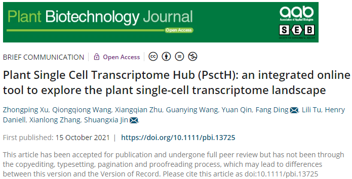
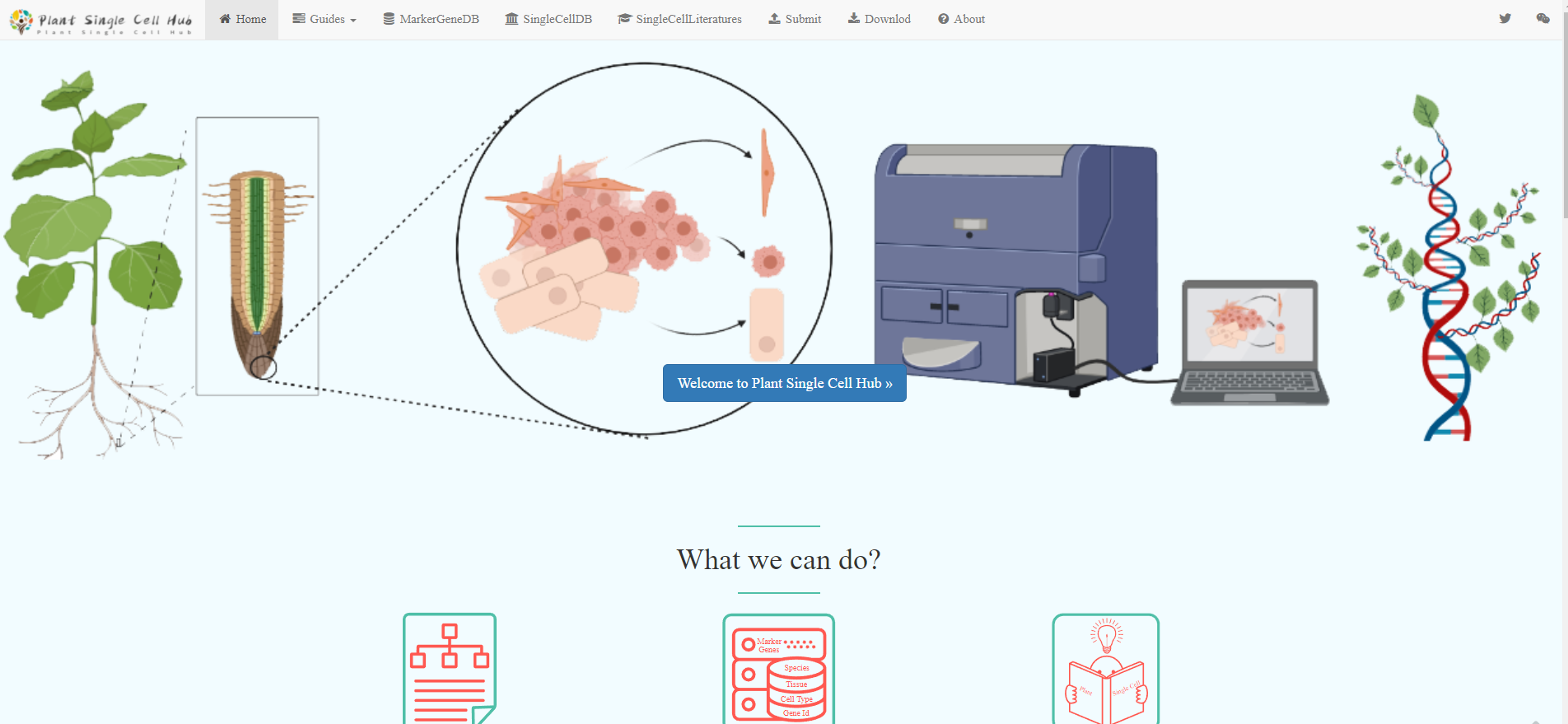
 图1. dCas9介导的基因调控系统。(Cell. 2013 Jul 18; 154(2): 442–451)
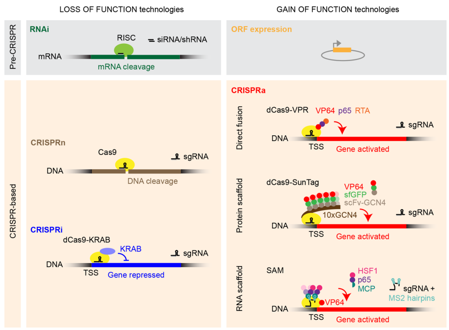 图2. 功能缺失或功能获得系统示意图。(ACS Chem Biol. 2018 Feb 16;13(2):406-416)
 作者将57个人的KRAB结构域融合到dCas9的N端,并用慢病毒感染法检测它们被招募到两个不同的含报告基因结构中时的活性。其中一种方法是将dCas9-KRAB融合靶向到SV40启动子上的两个位点,该启动子驱动人类胚胎肾器官293T细胞(HEK293T)中绿色荧光蛋白(EGFP)的表达。在另一组实验中,dCas9-KRAB融合蛋白靶向K562细胞的PGK1-EGFP报告基因下游的7×TetO阵列上(图3)。且两种报告细胞系均来自单细胞克隆,以确保报告基因和gRNA表达水平的一致性。
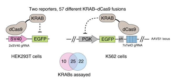 图3. KRAB结构域筛选系统。
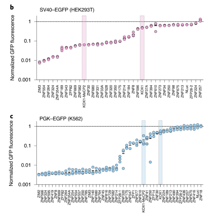 图4. 不同dCas9-KRAB融合体对靶标基因的沉默效果。
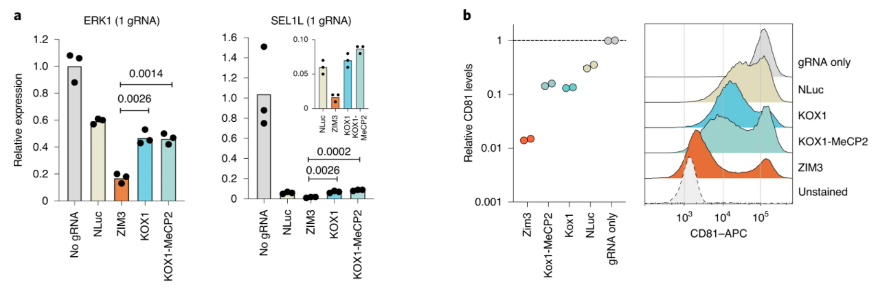 图5. 靶向ERK1,SEL1L和CD81启动子和相应基因的RT–qPCR表达水平。
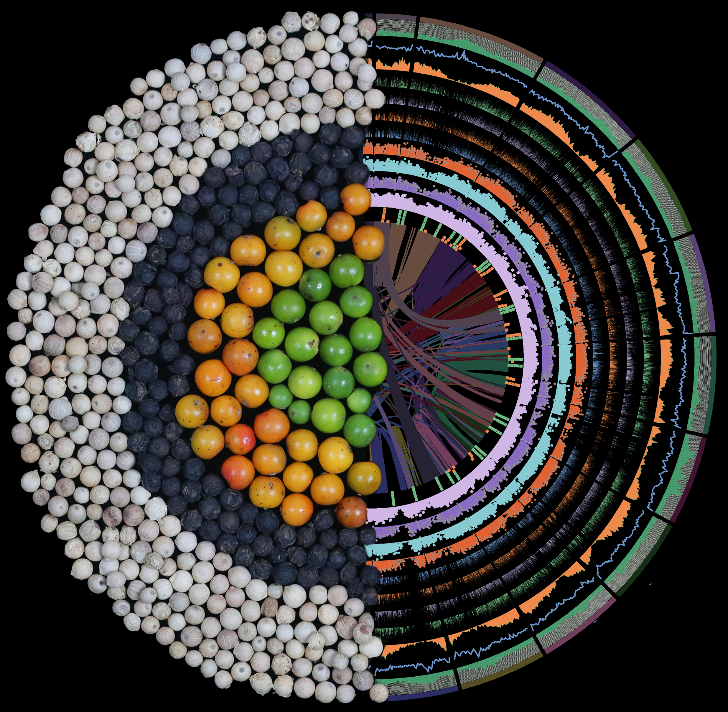
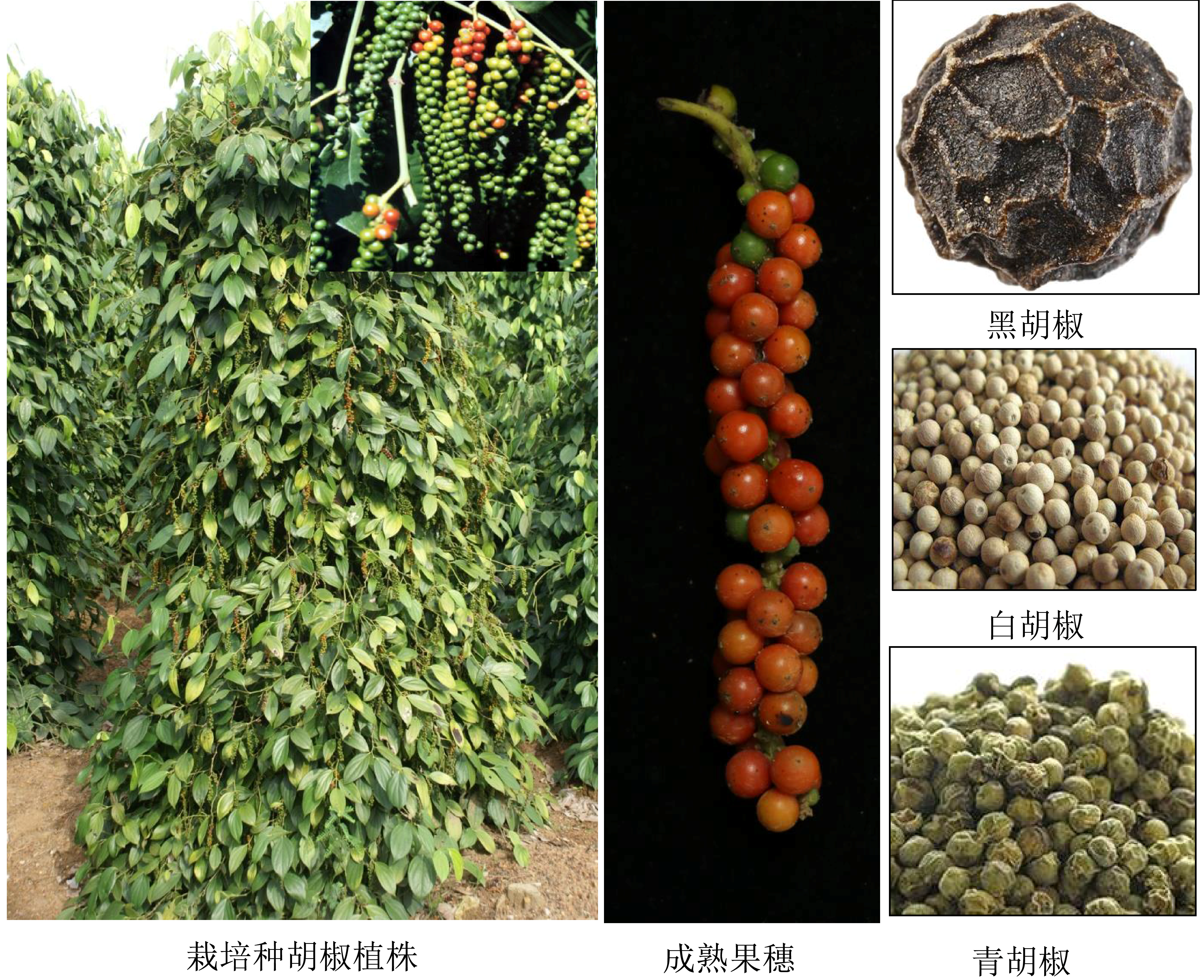

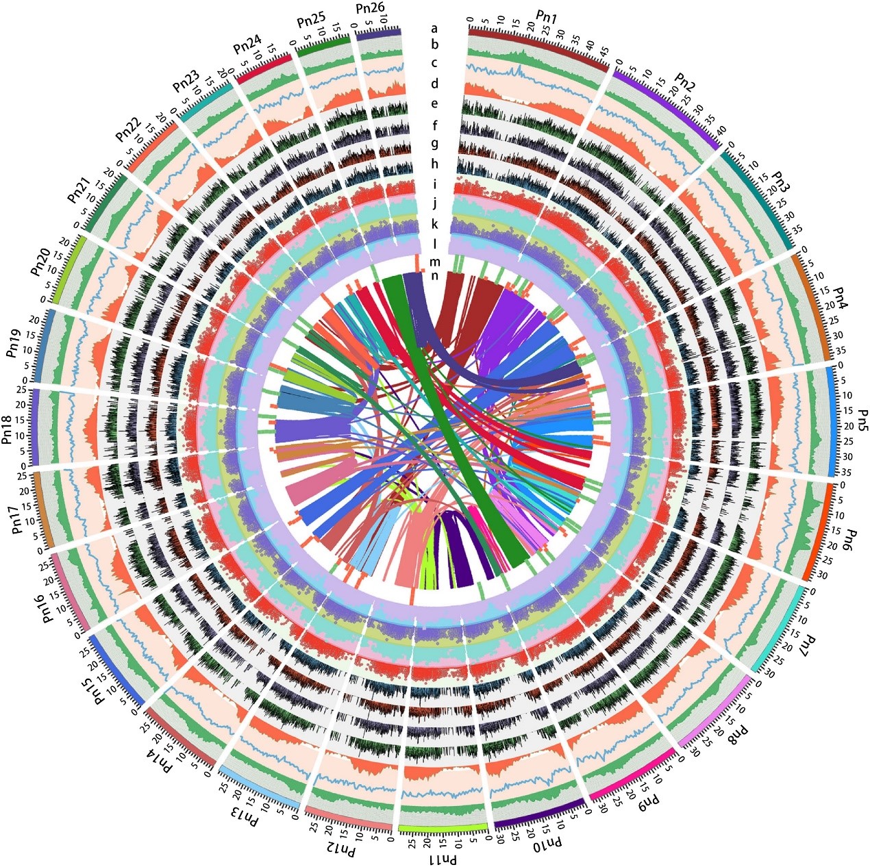
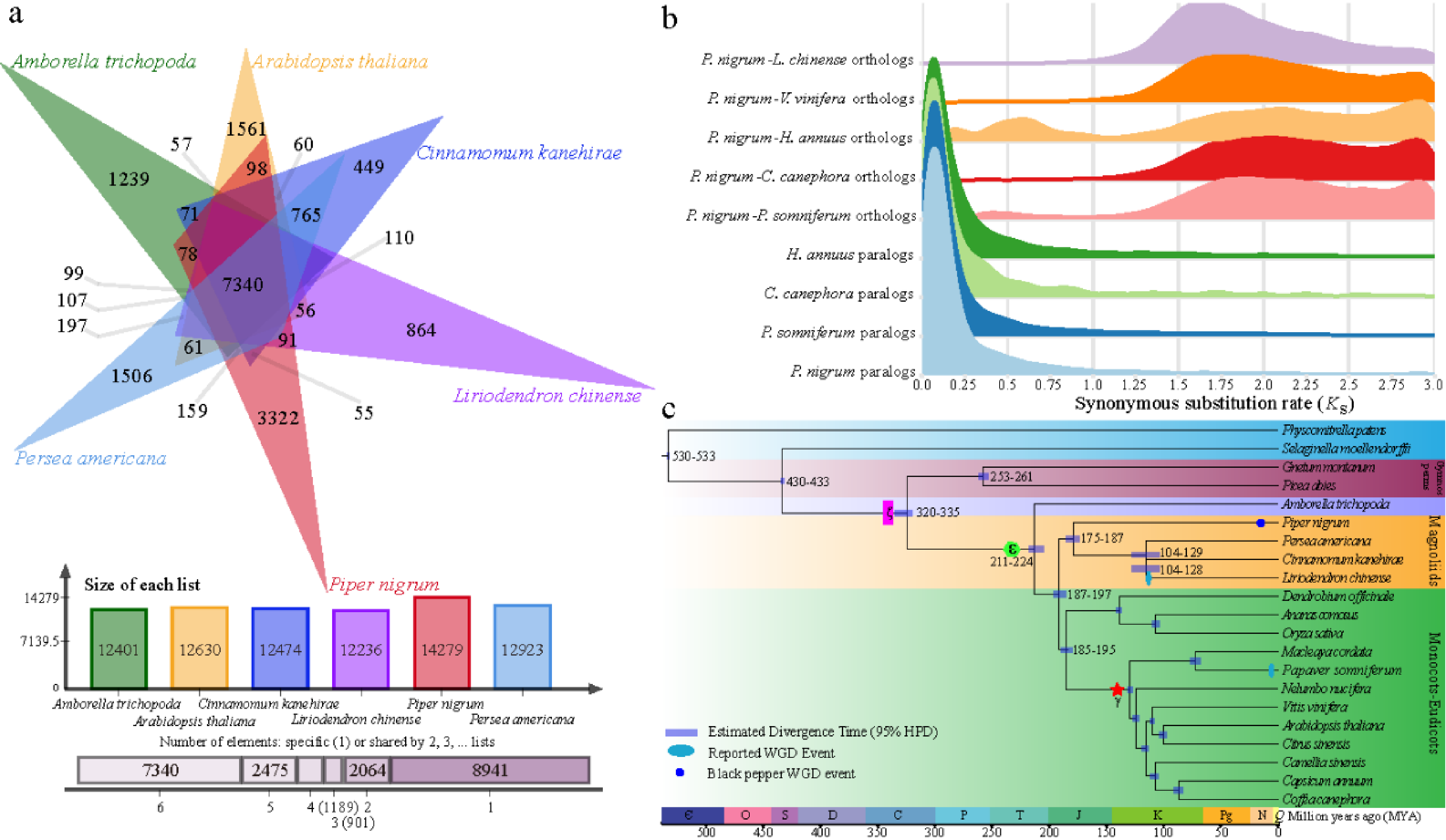
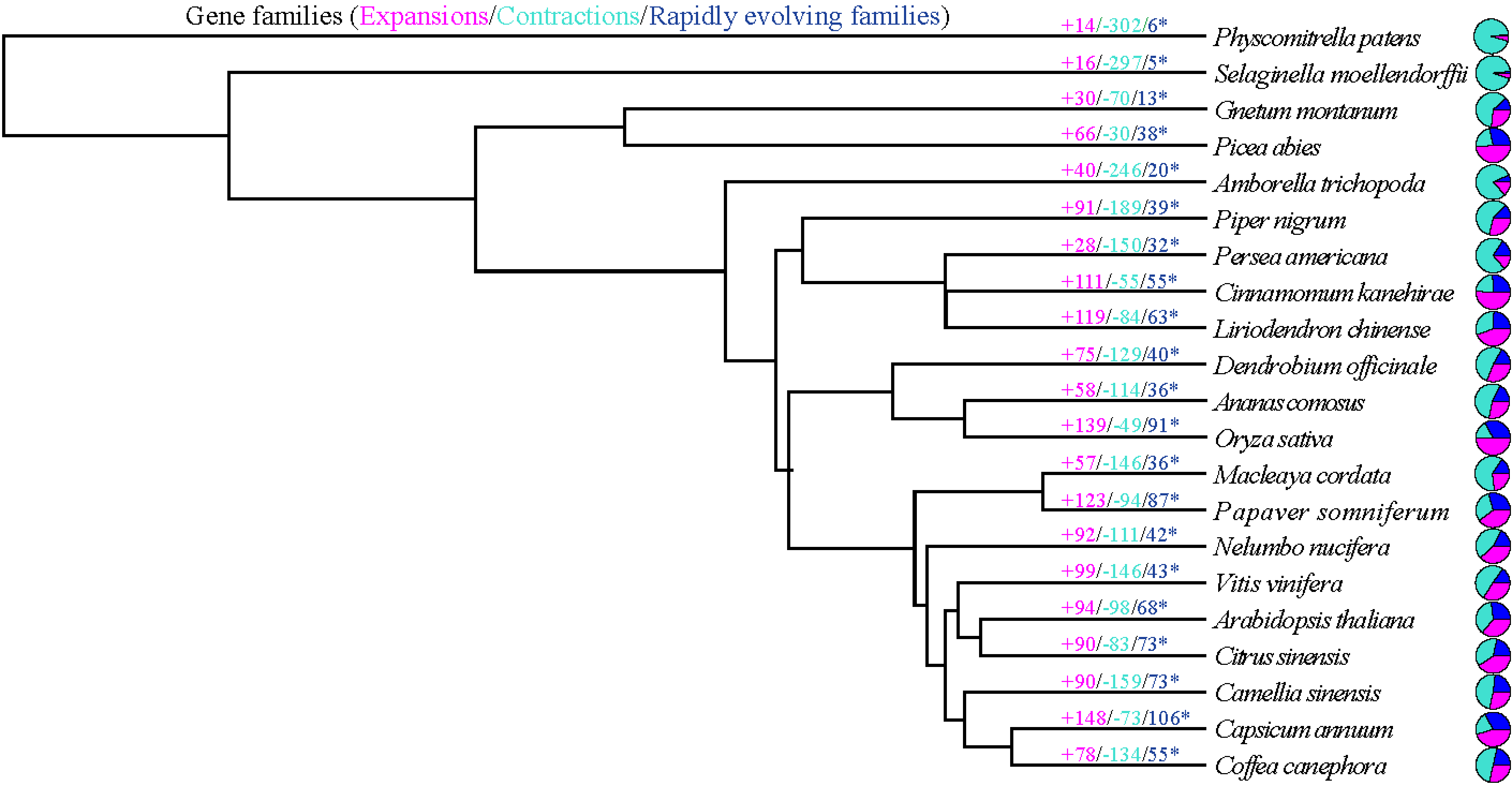
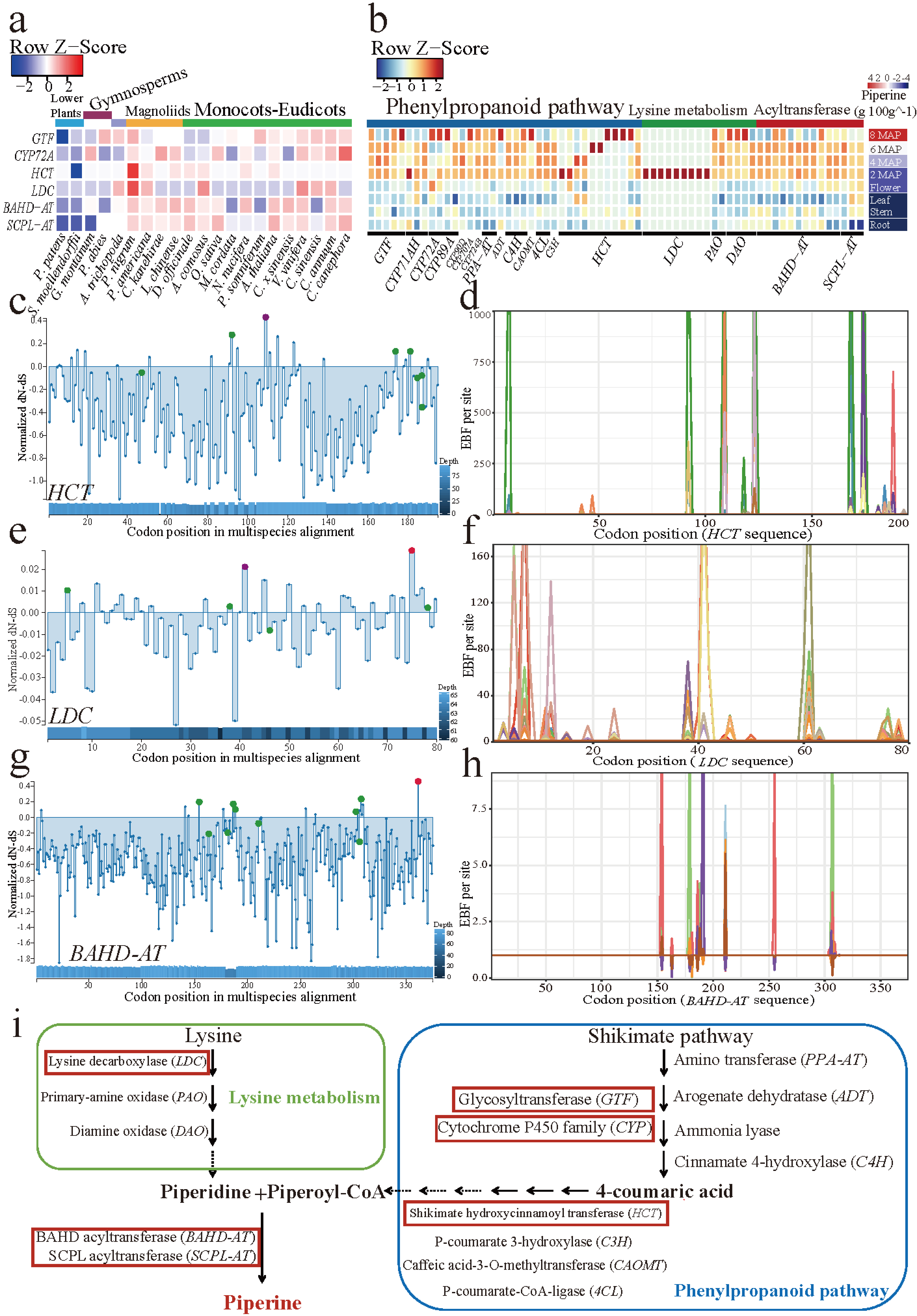
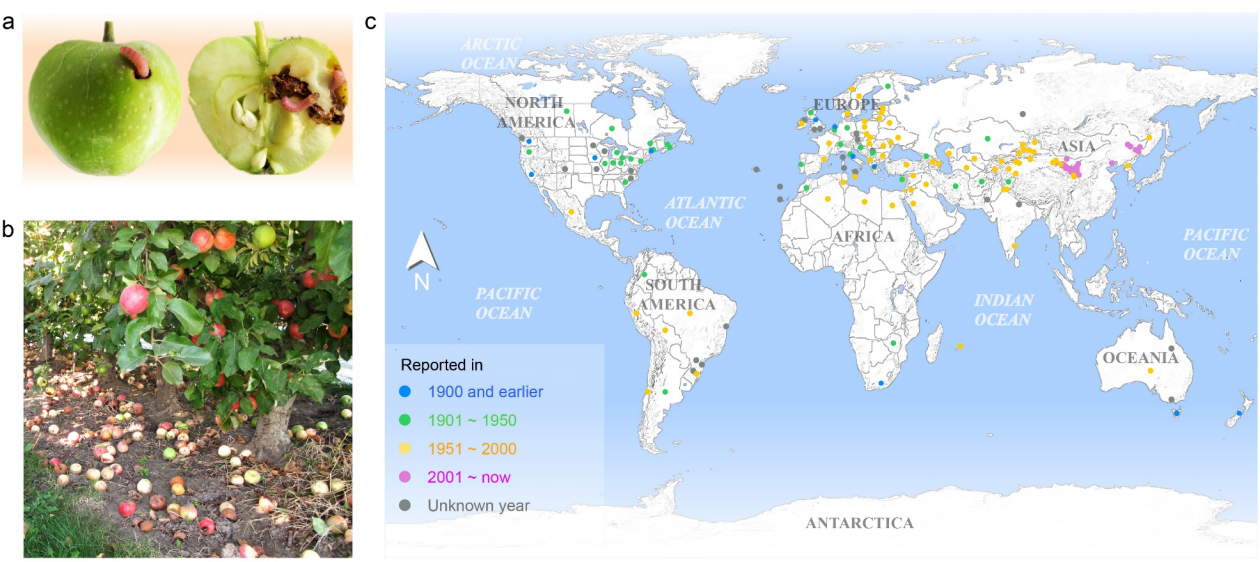
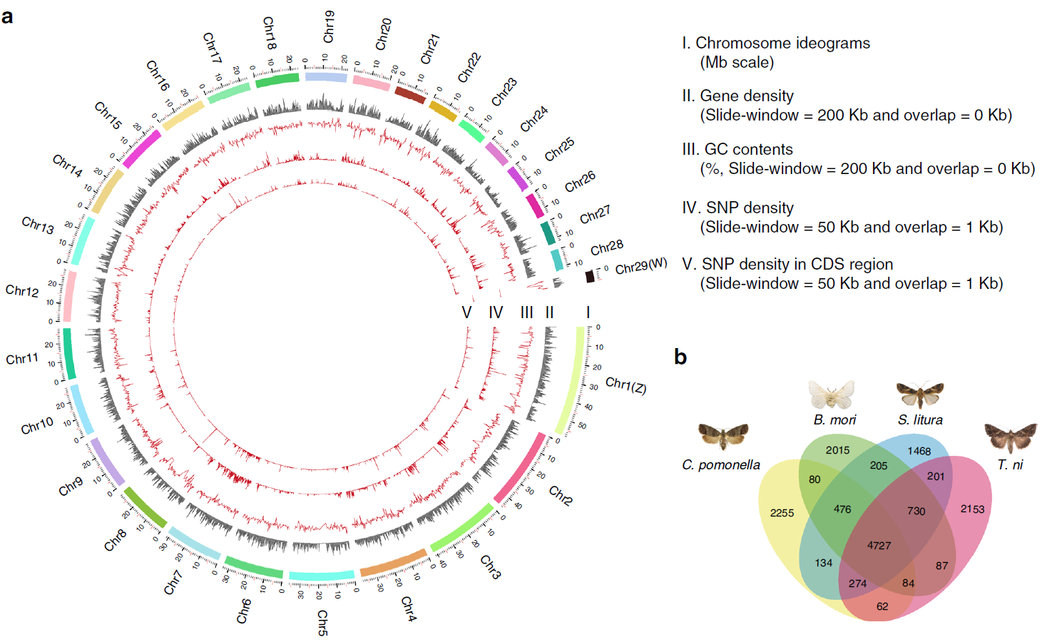
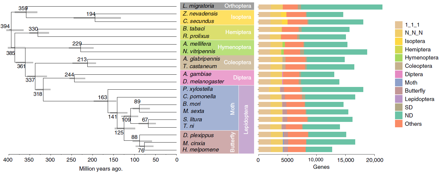
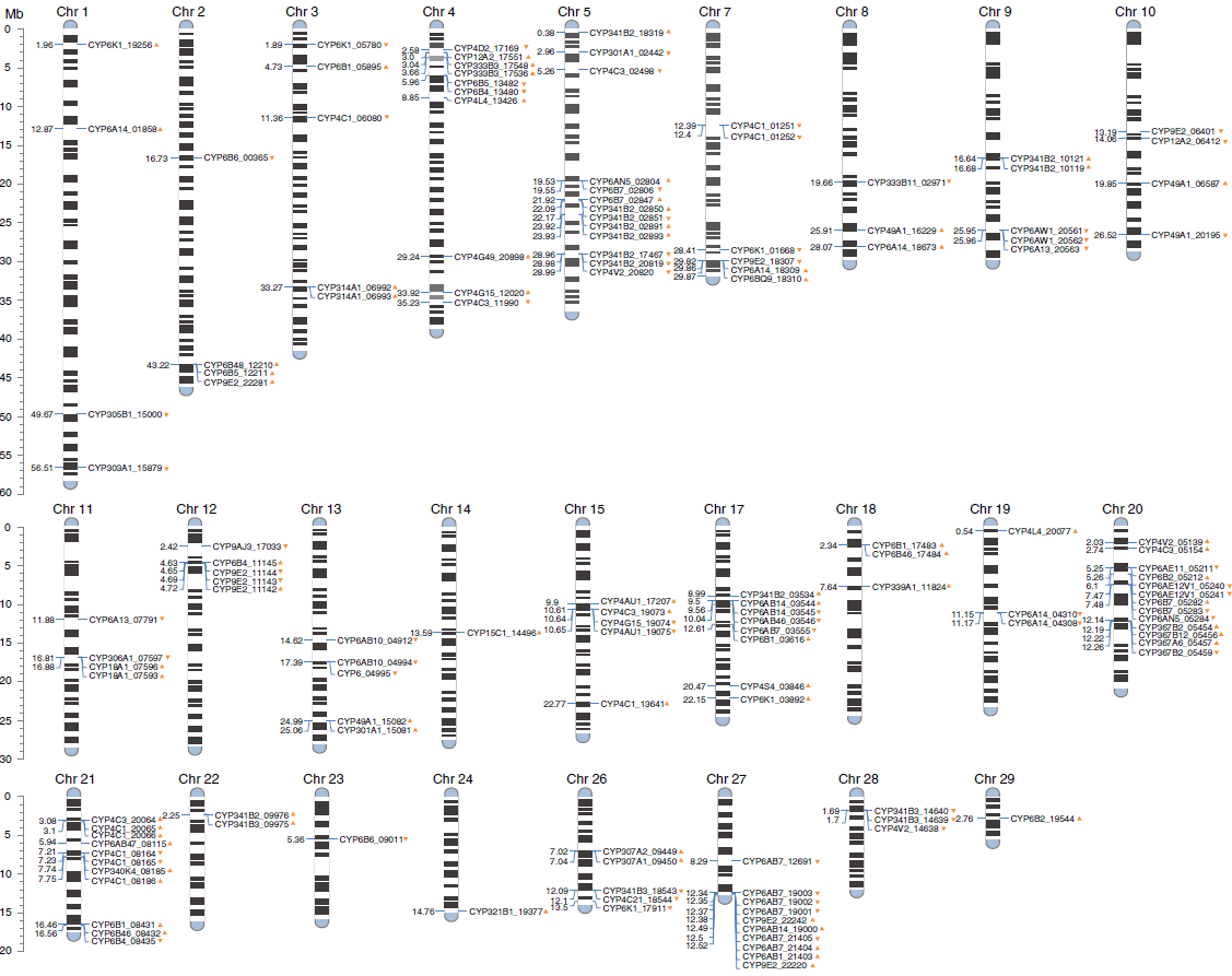
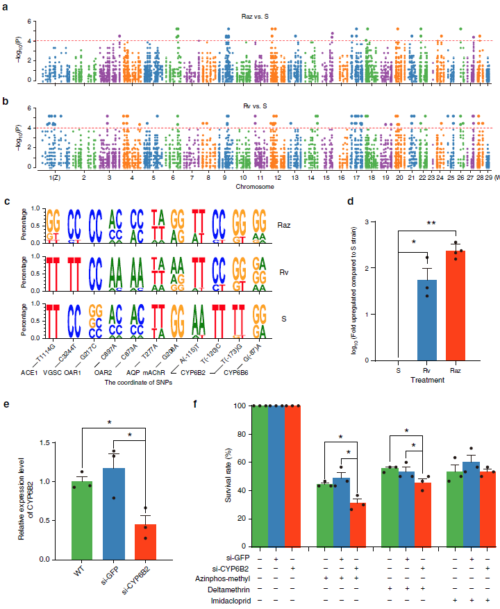


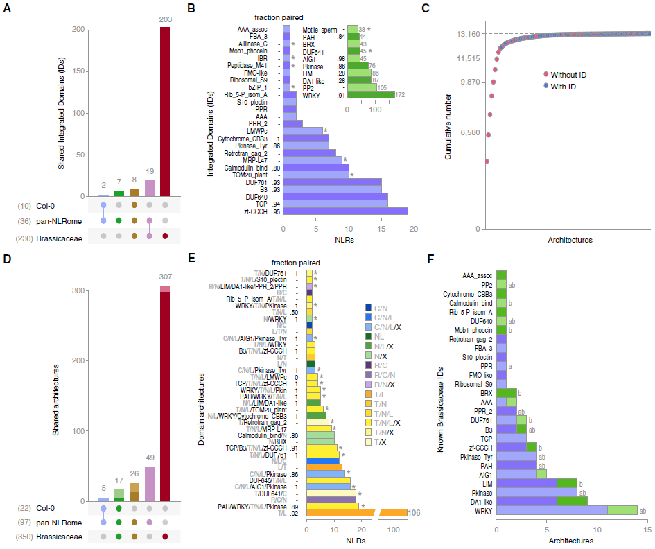
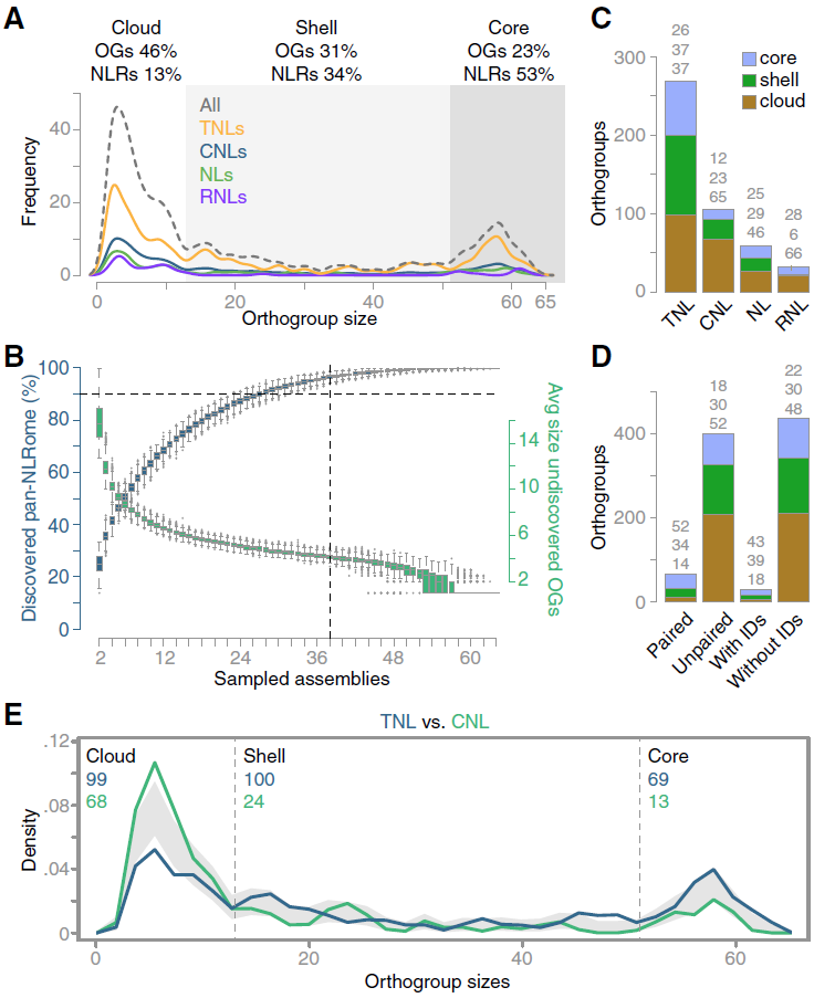
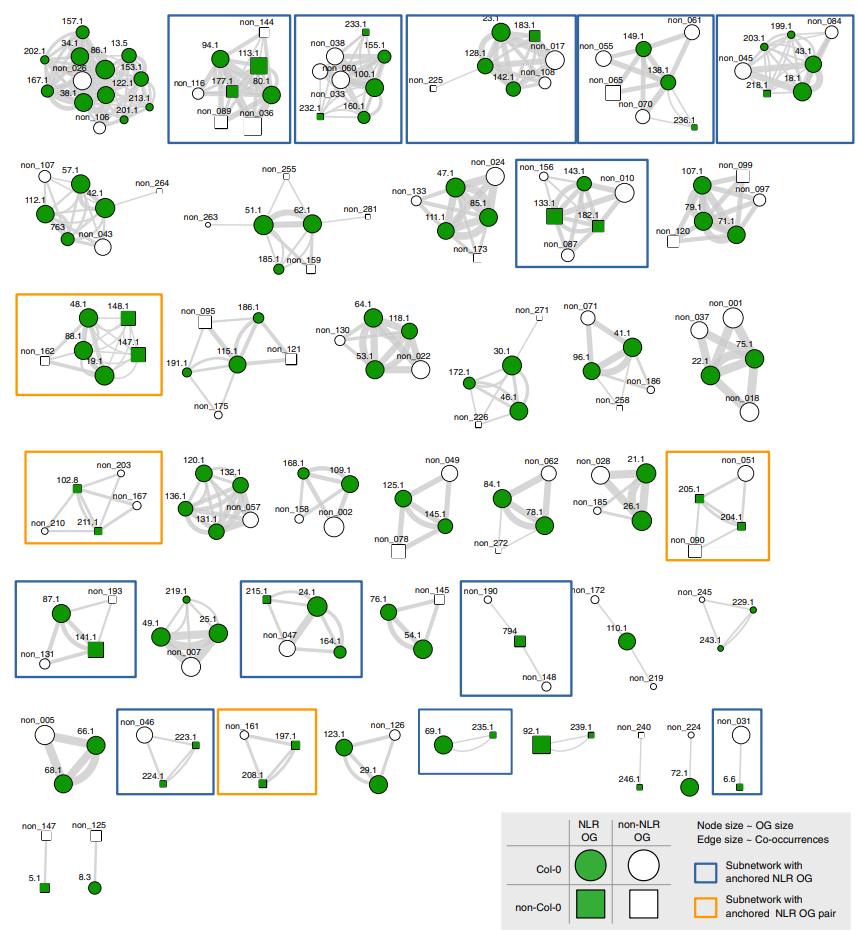
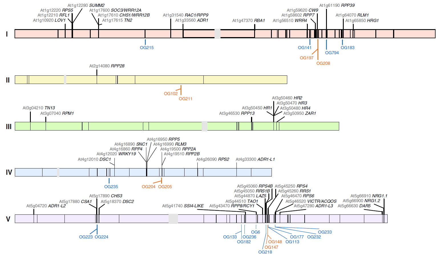
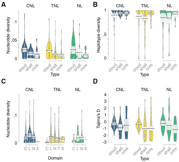


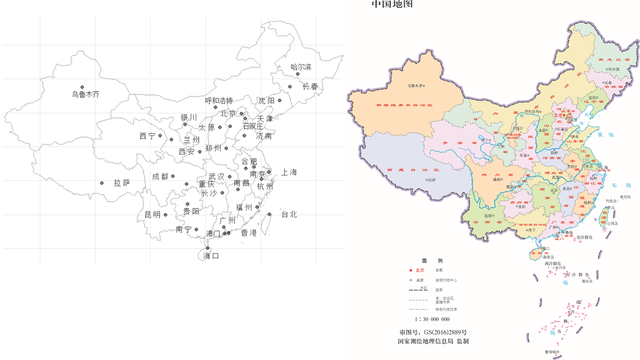
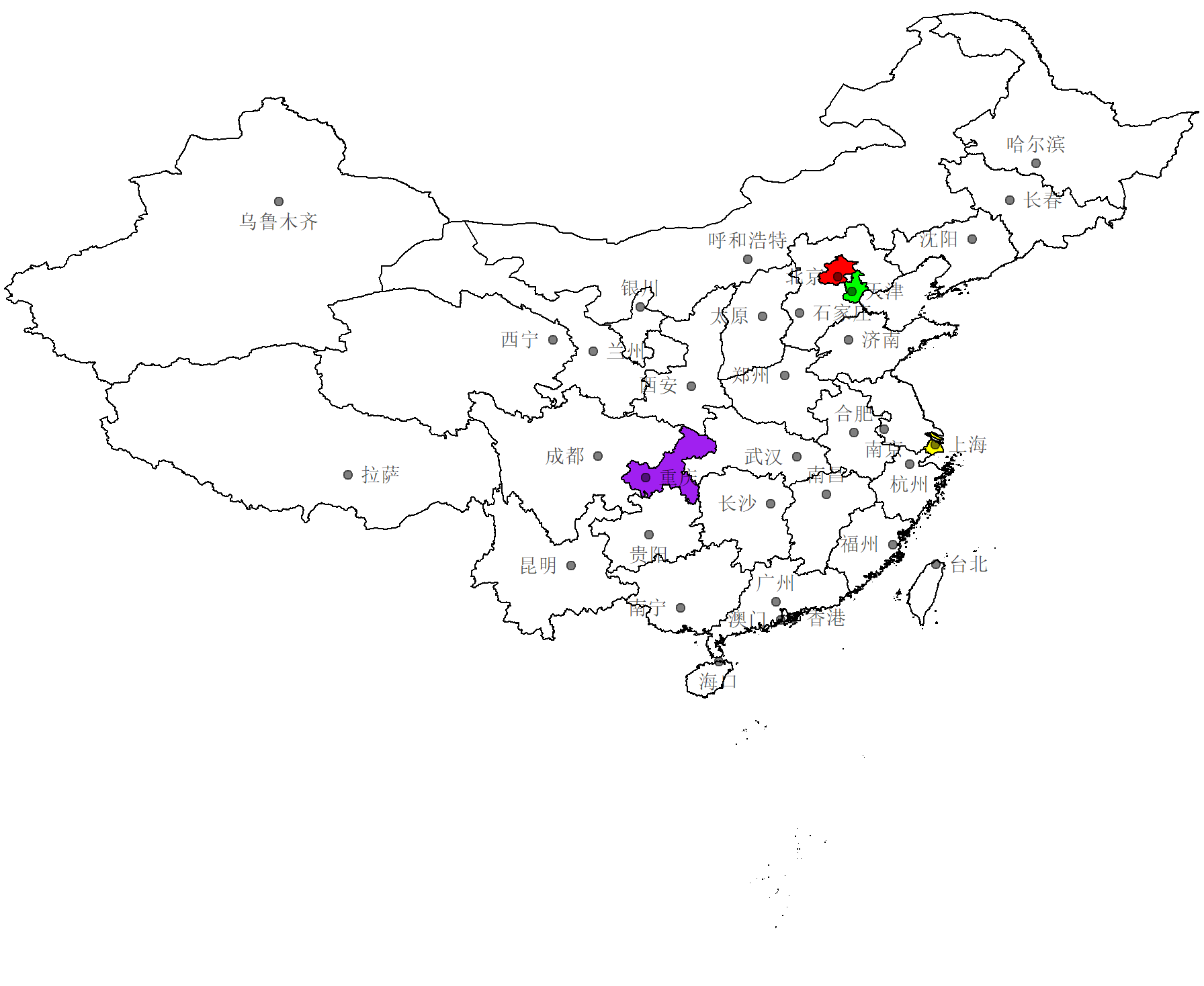
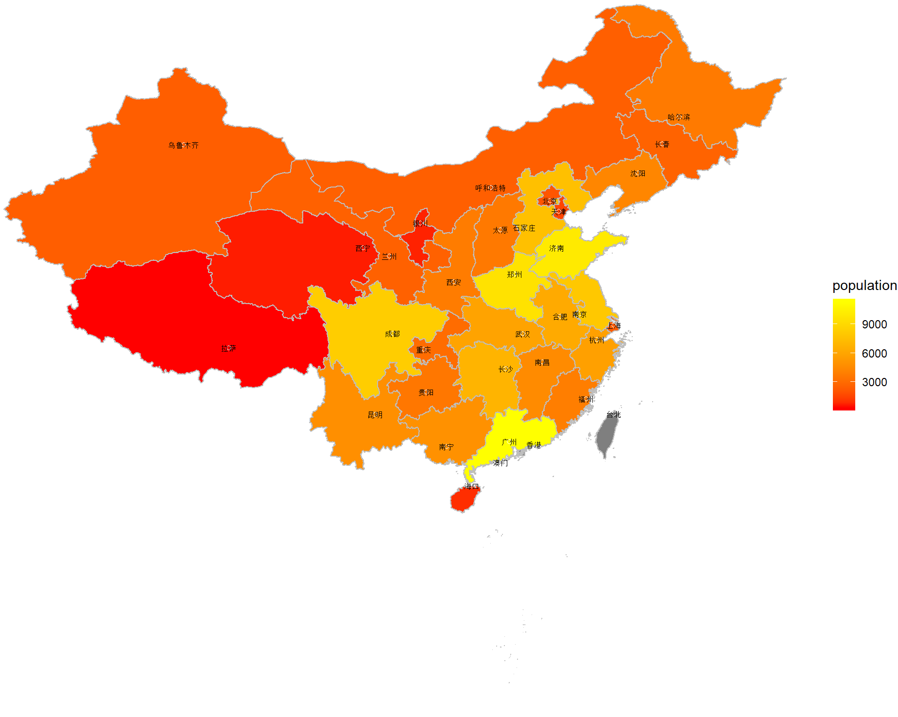
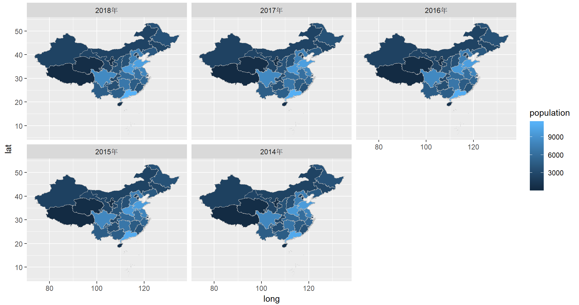
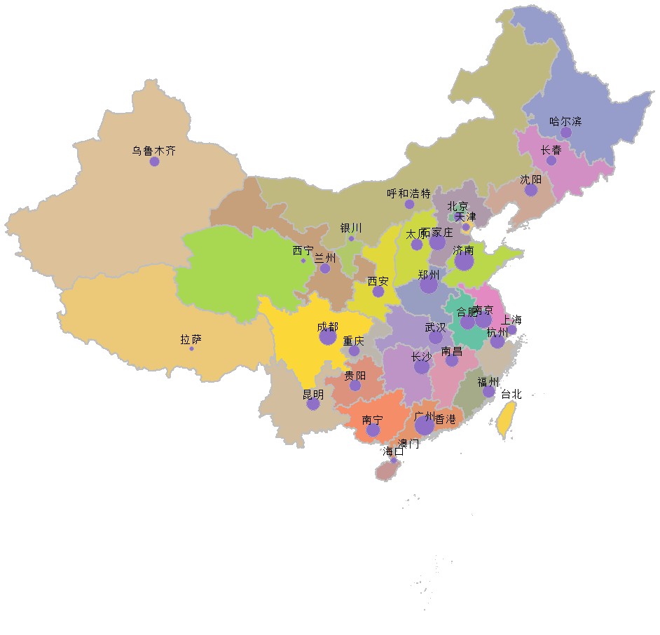


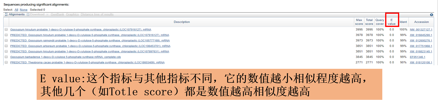

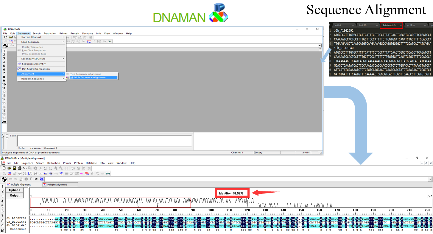
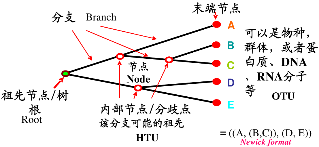
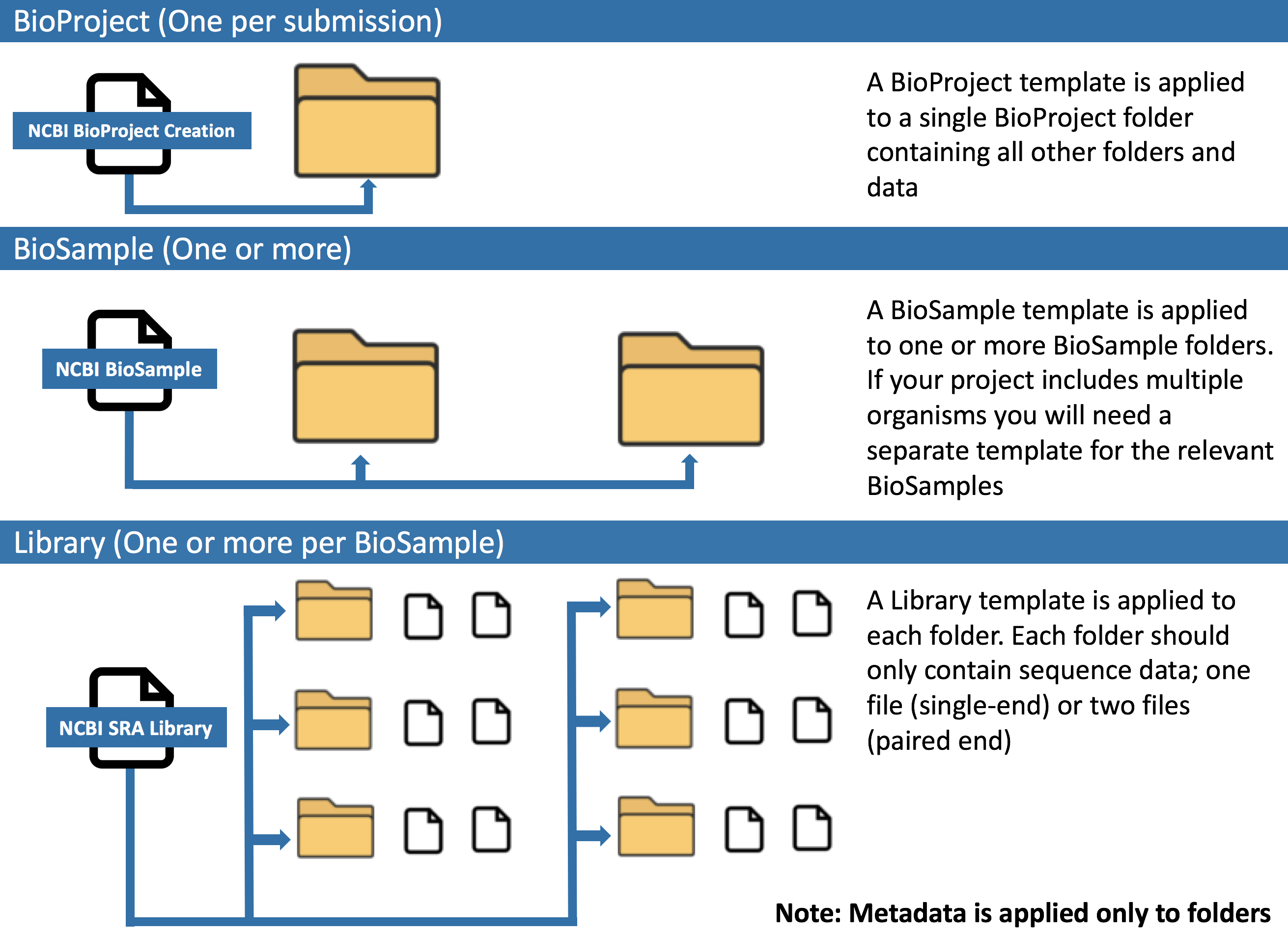
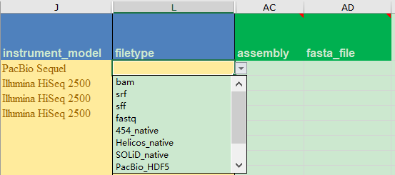
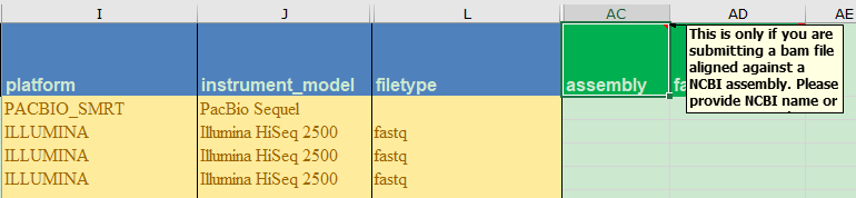
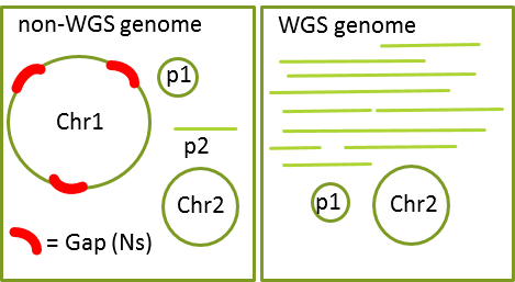
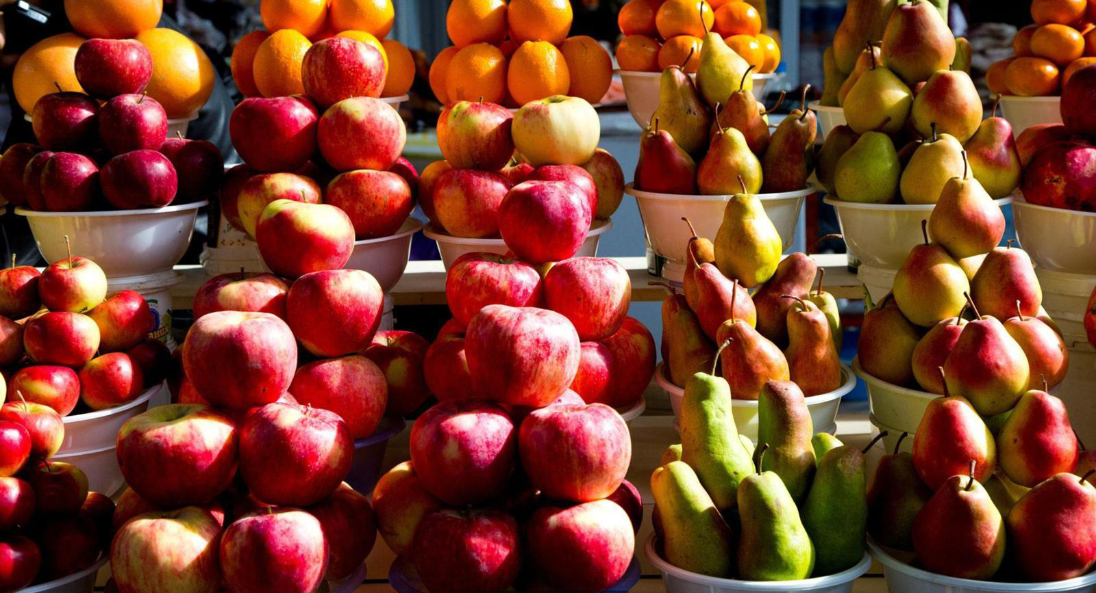

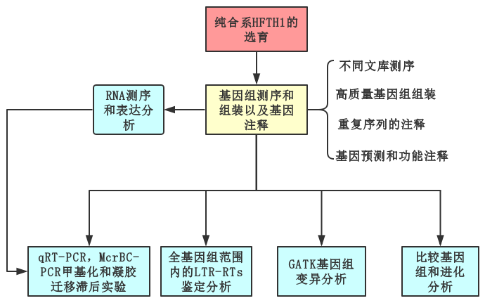
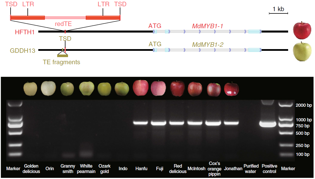


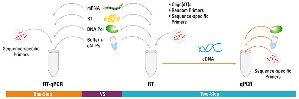

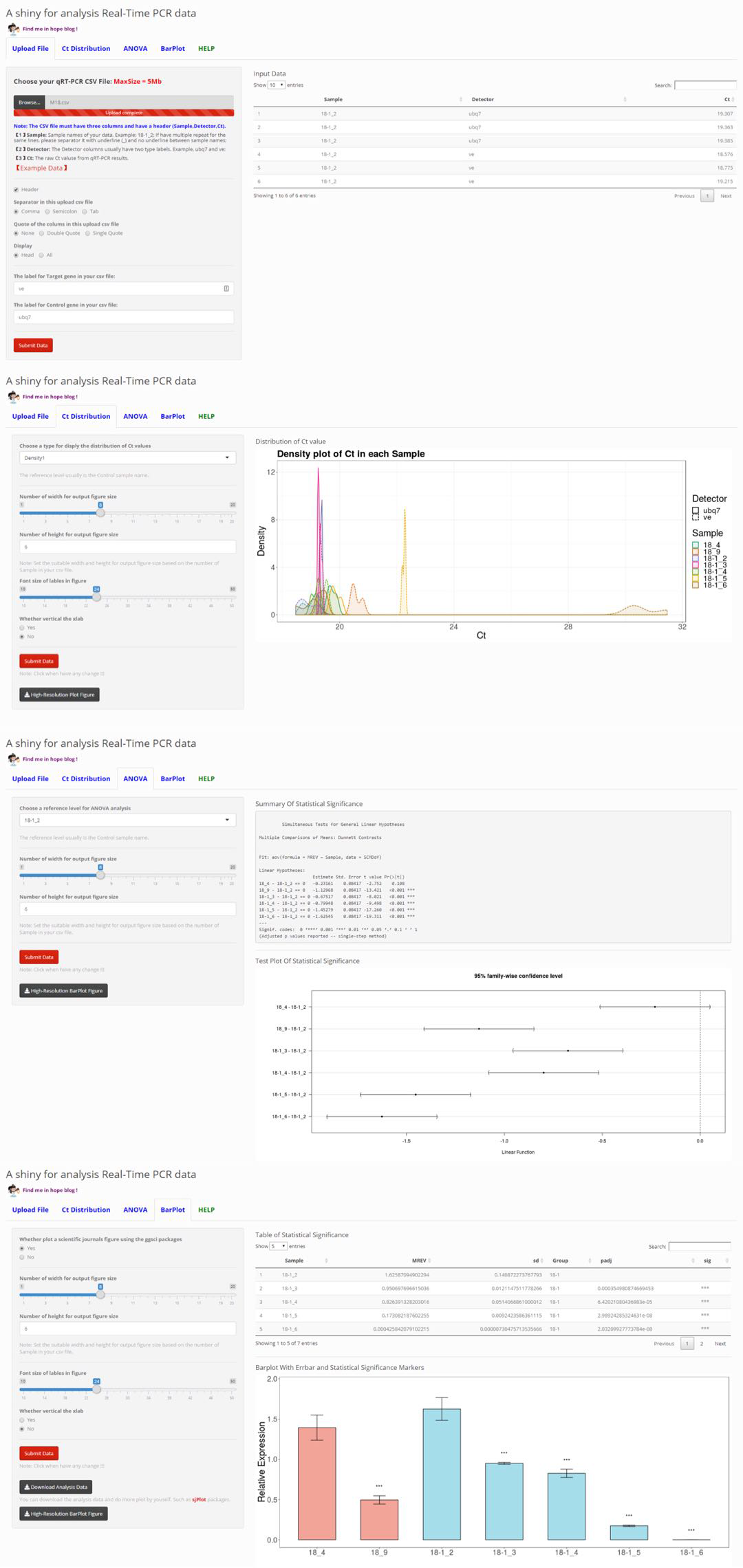
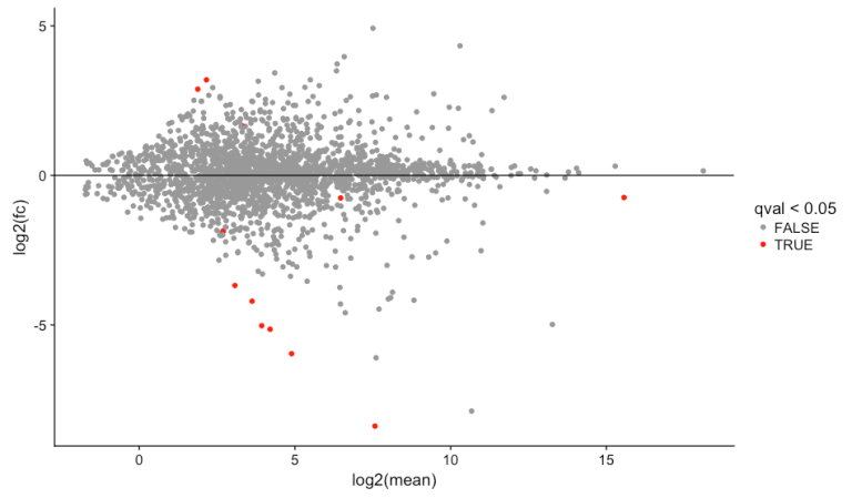
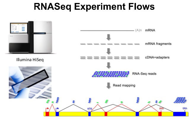
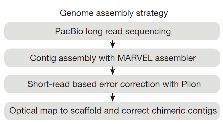
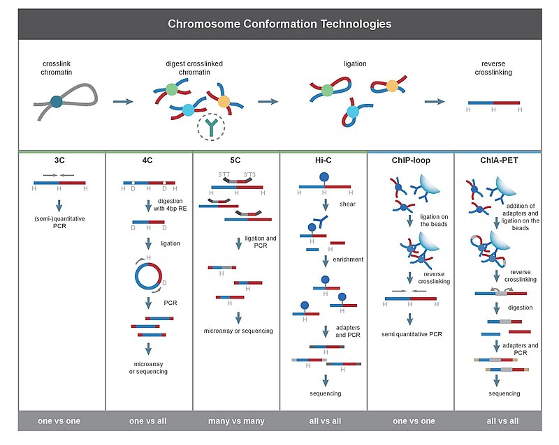
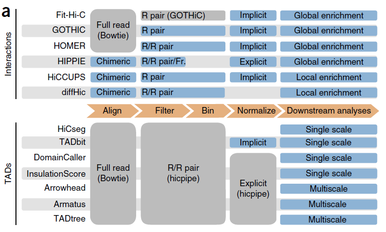
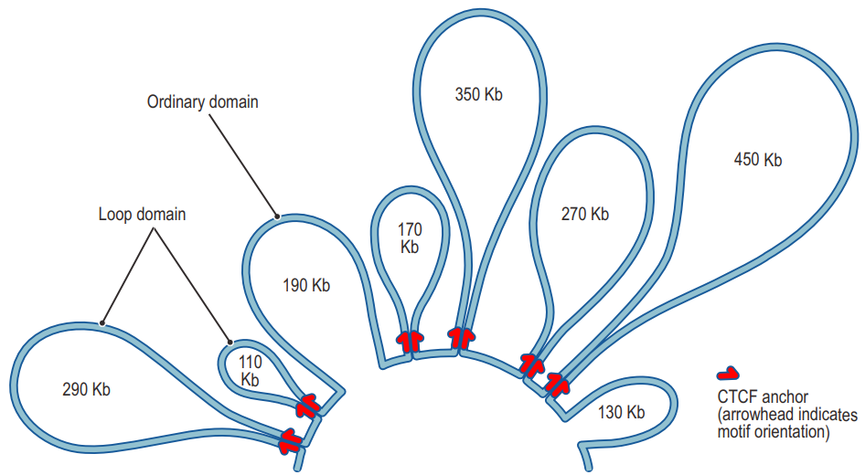


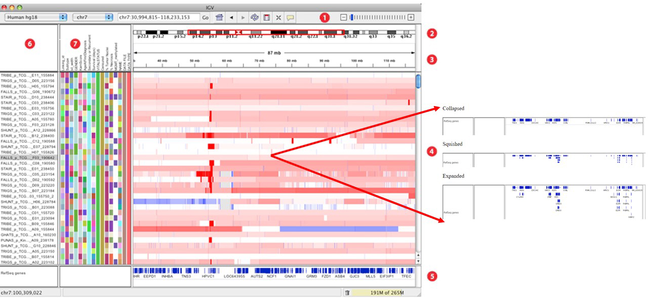
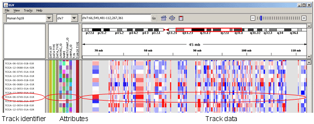
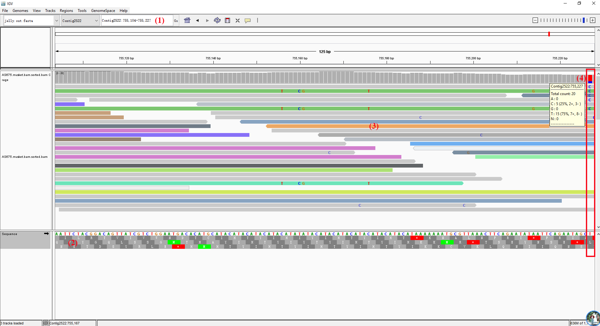
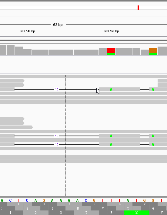
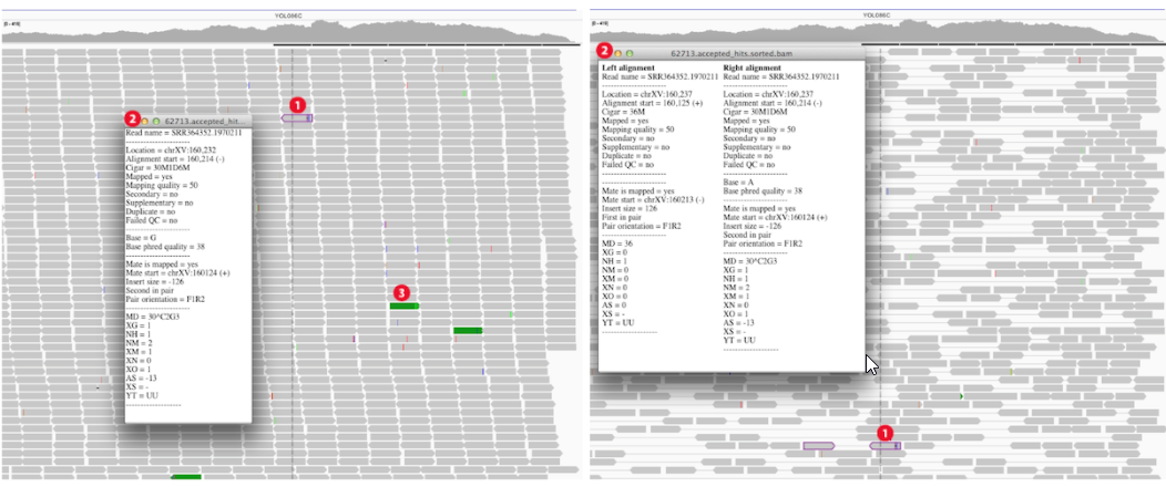
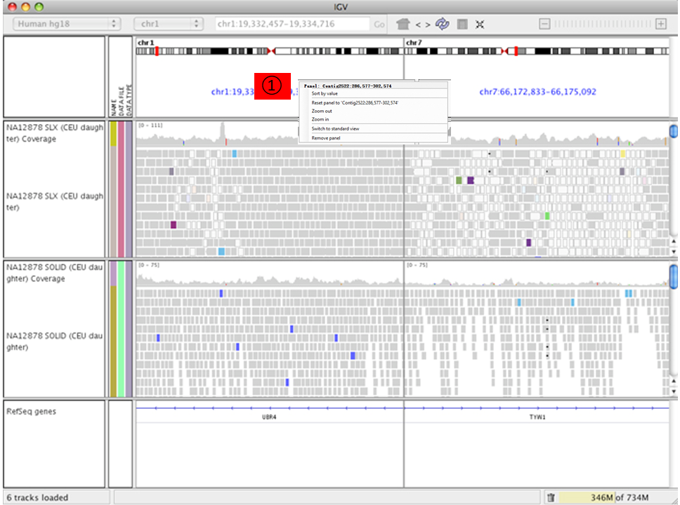
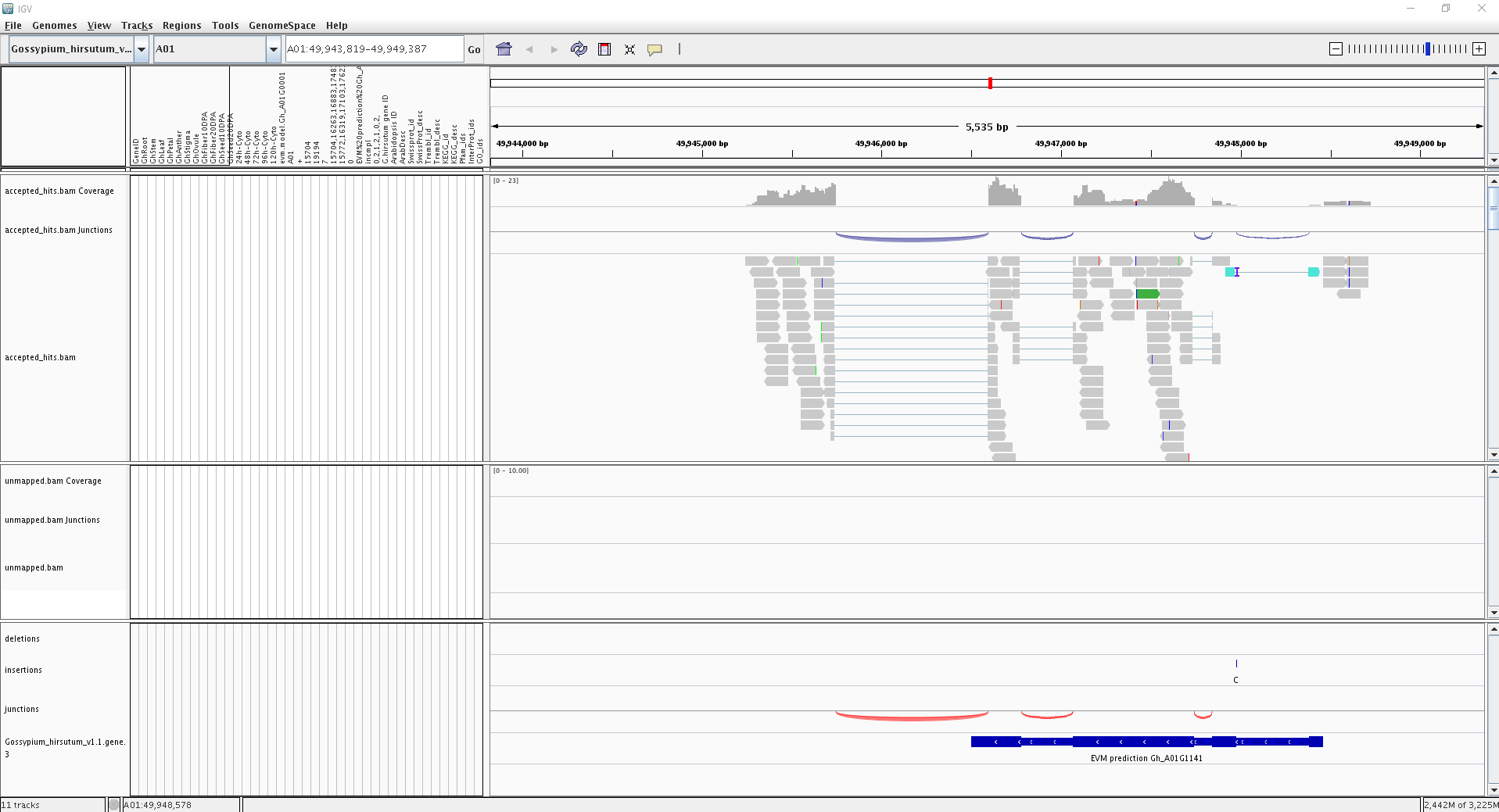


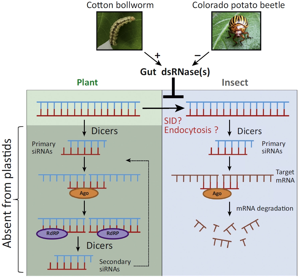


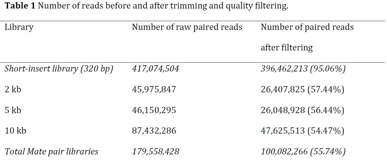
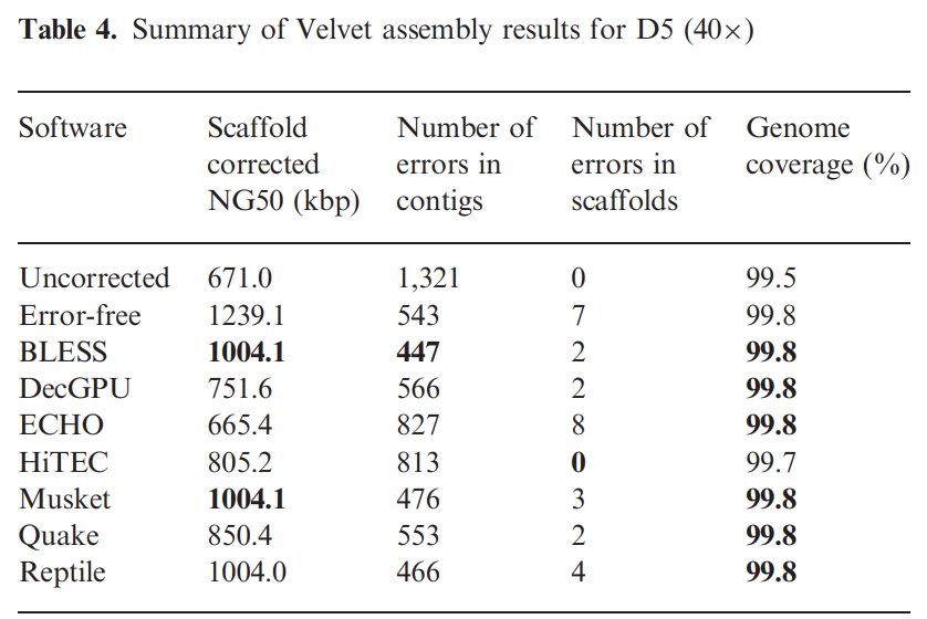


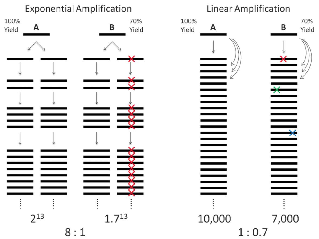
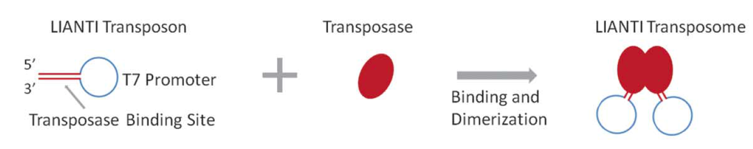
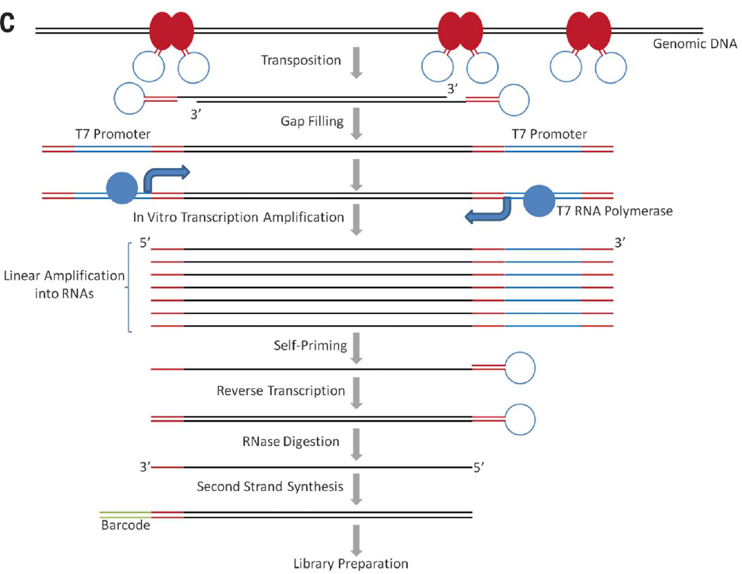
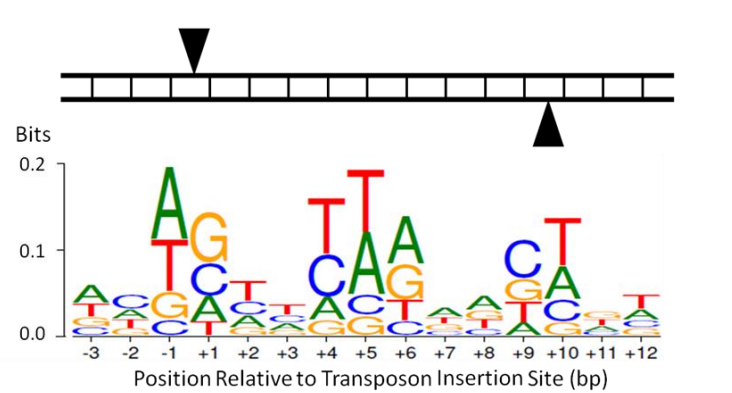
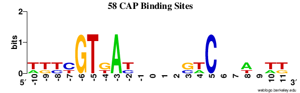
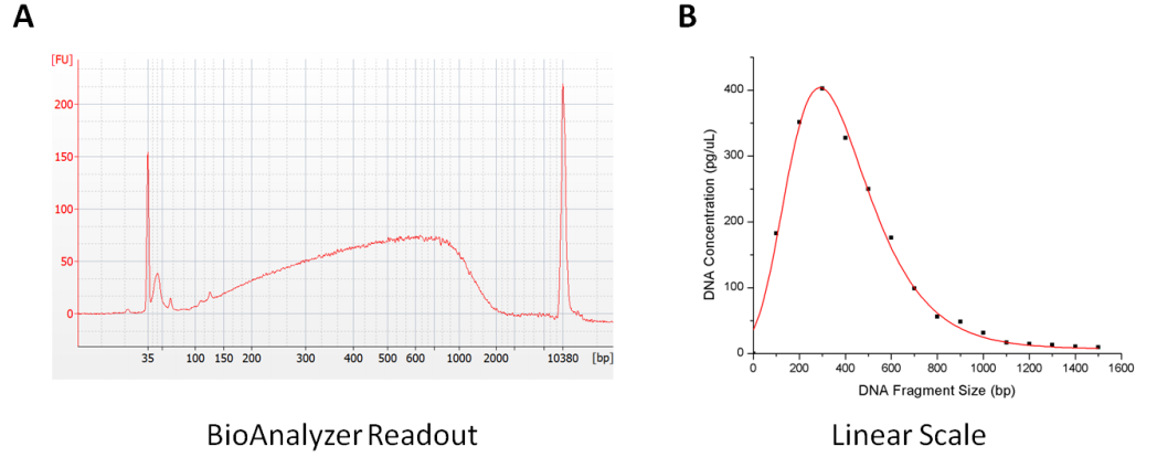
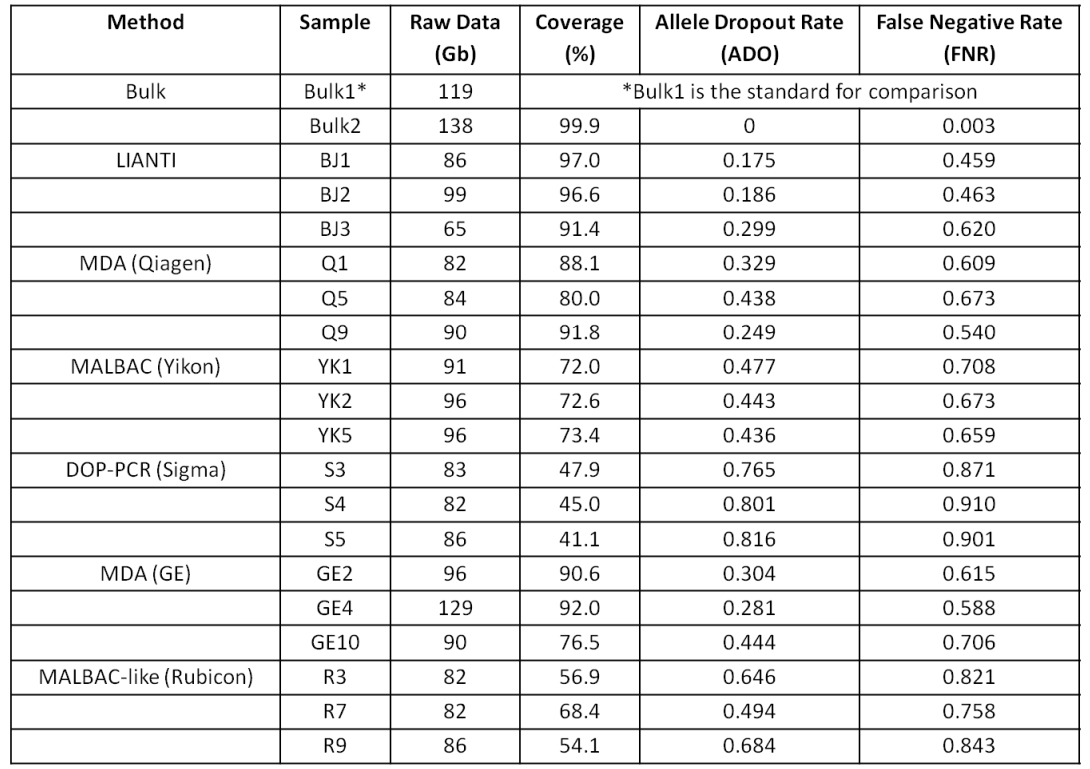
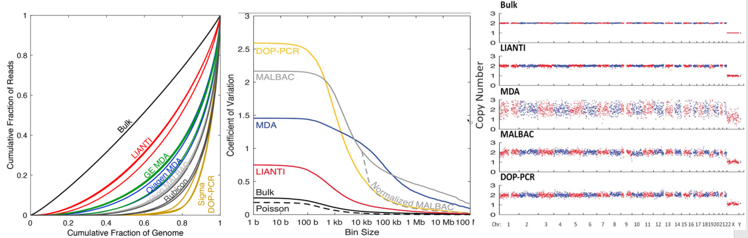
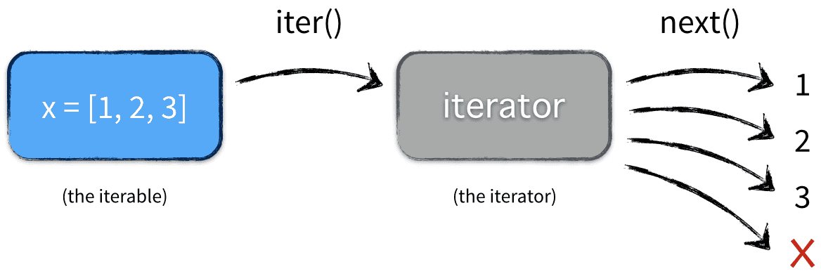
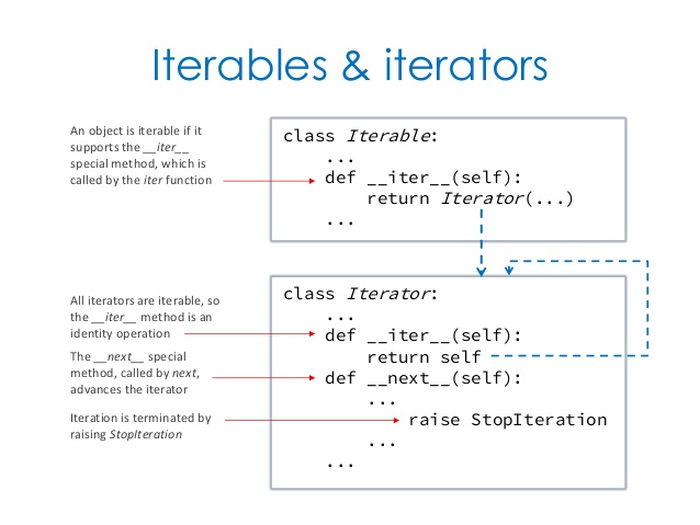
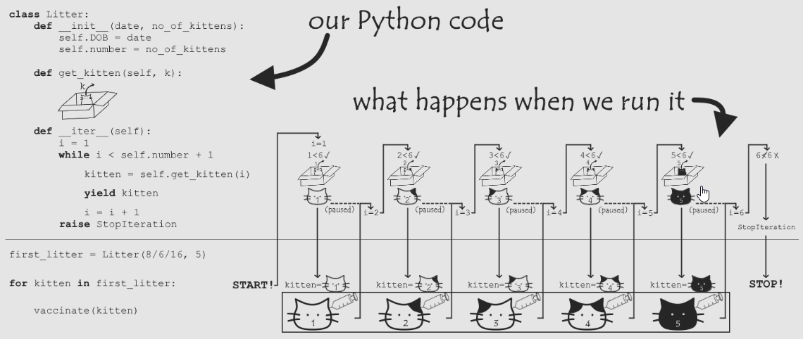


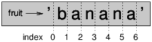
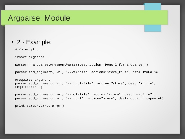
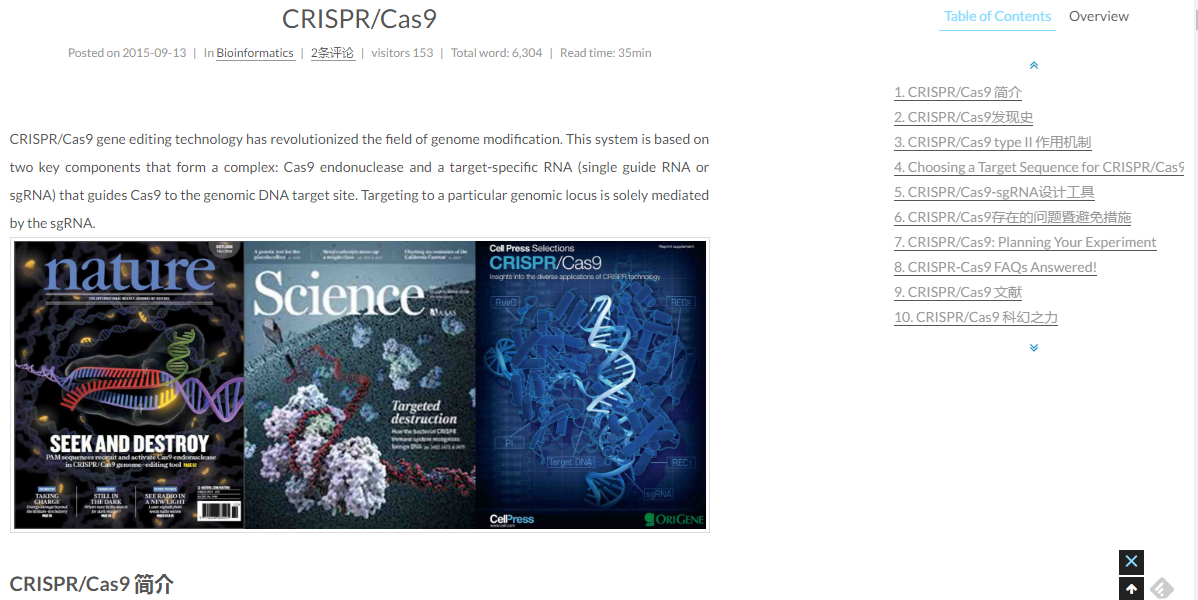
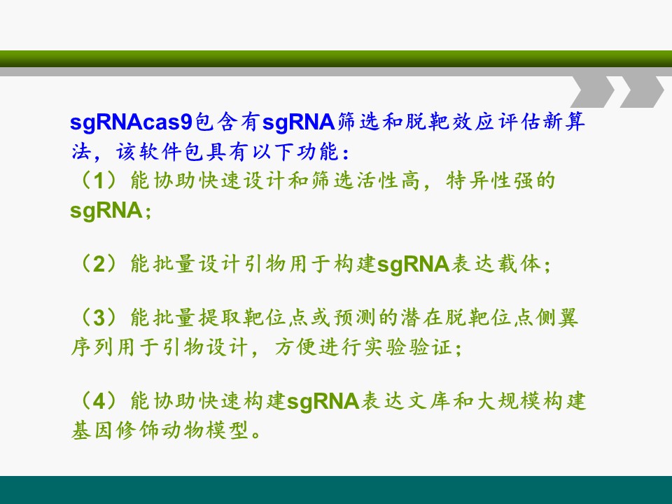


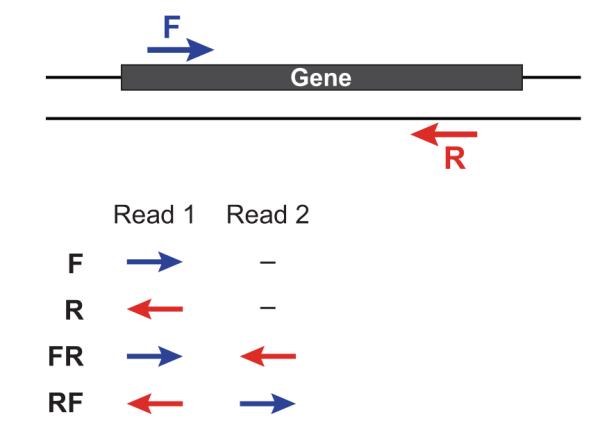
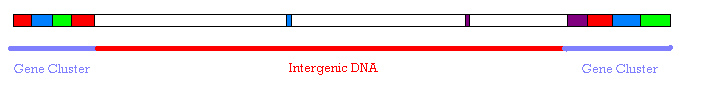
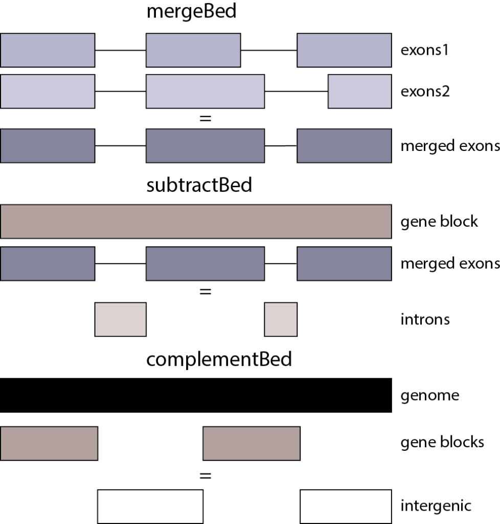
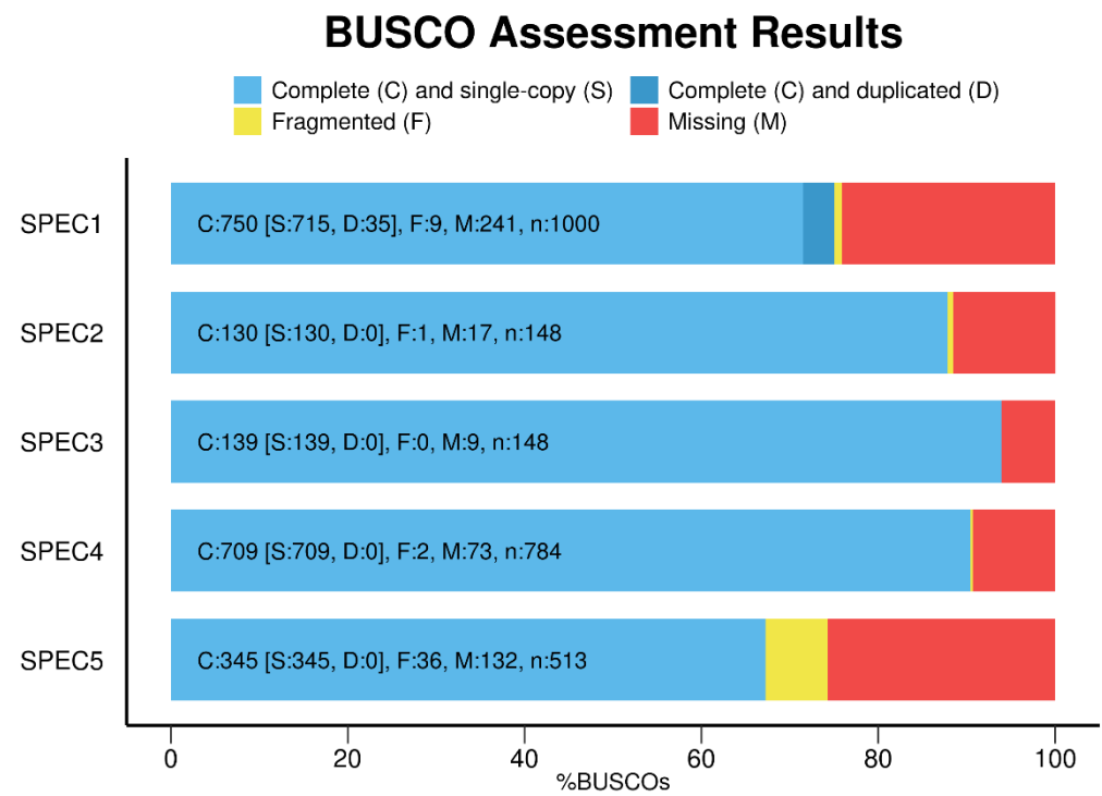
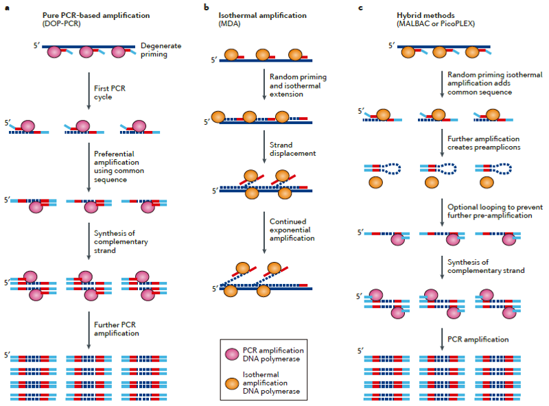
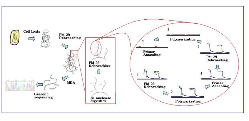
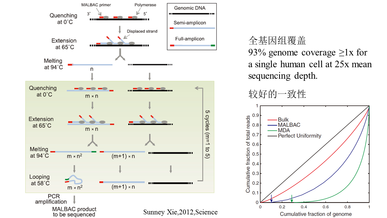
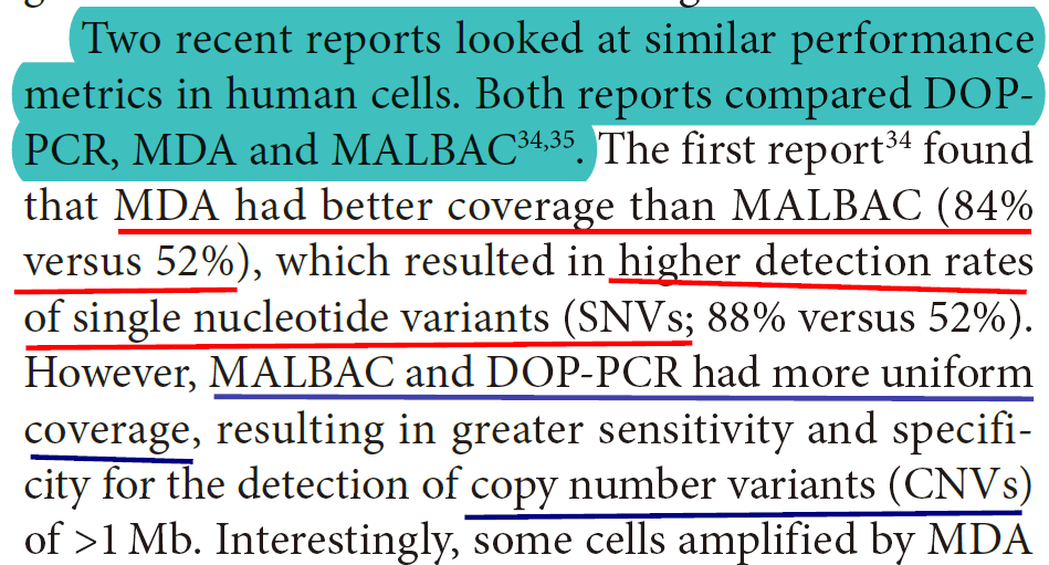
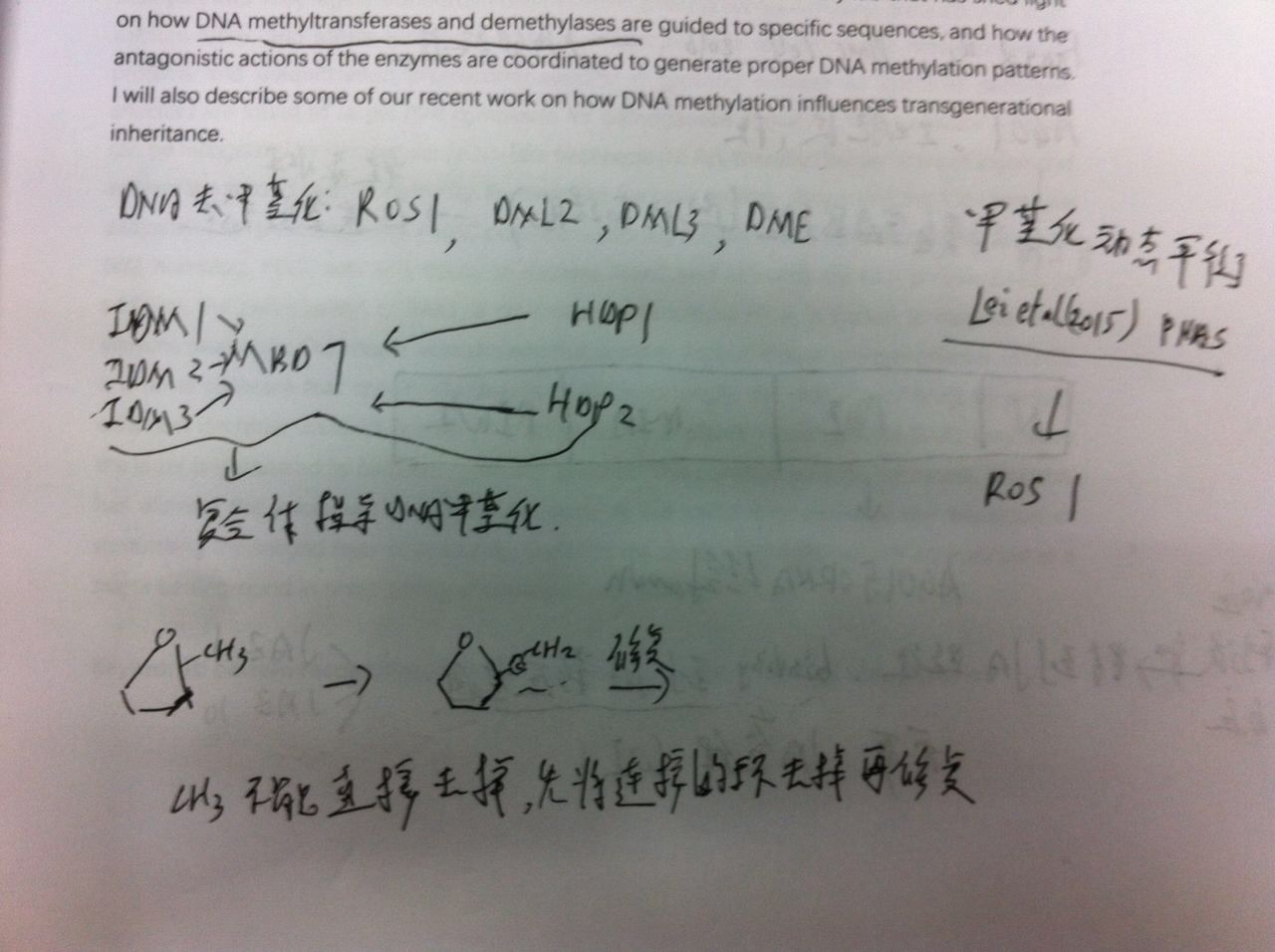

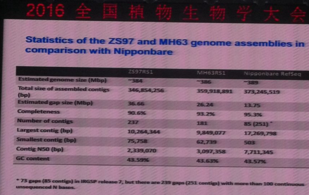
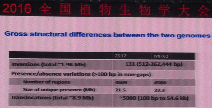
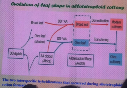

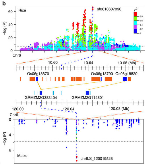
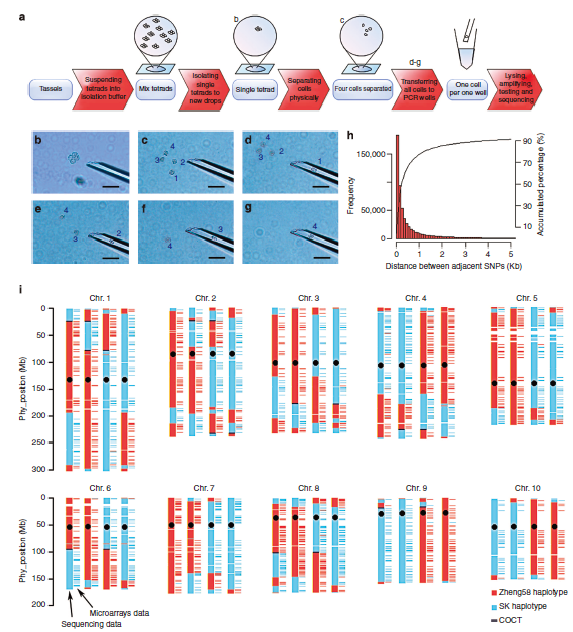
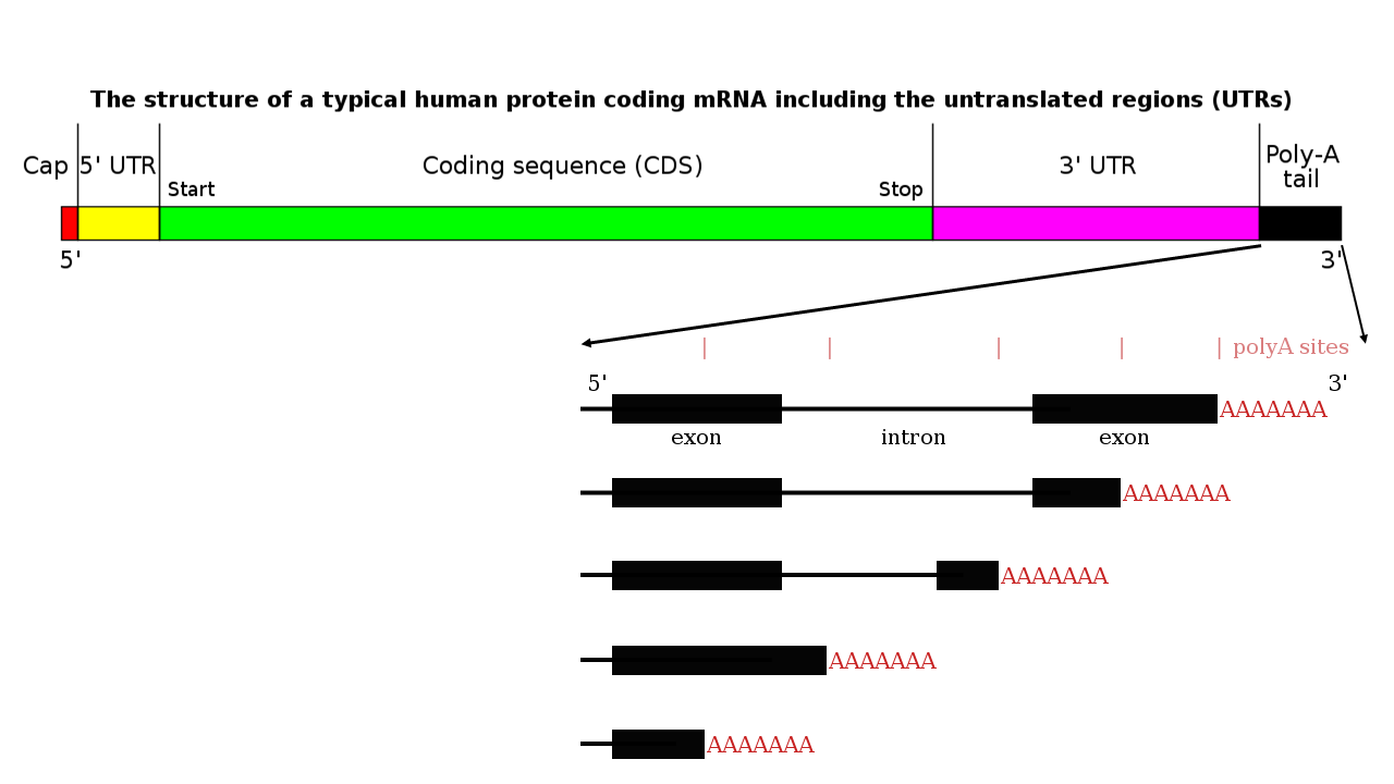
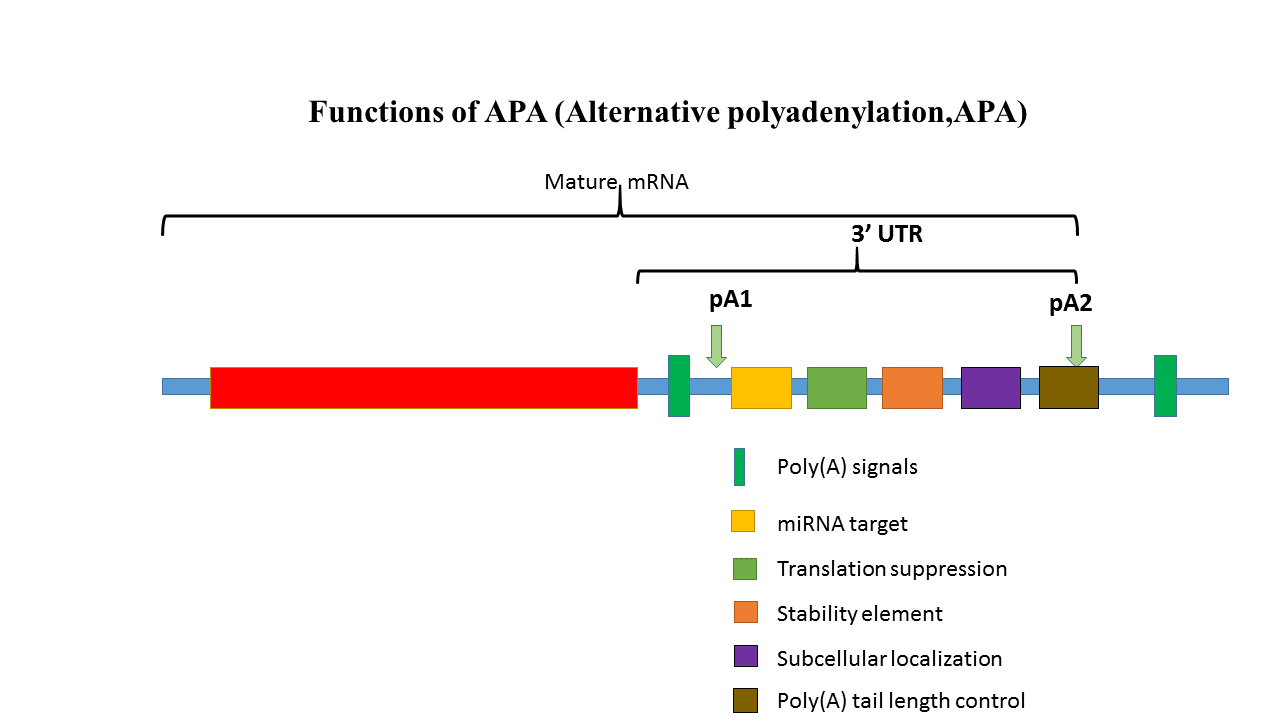
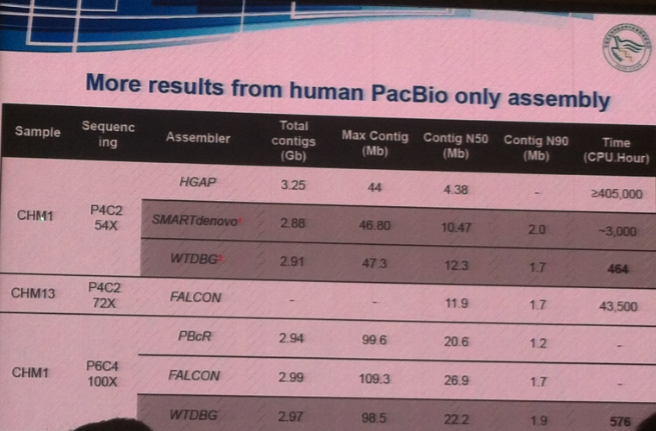
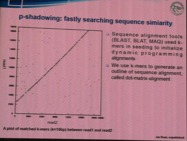
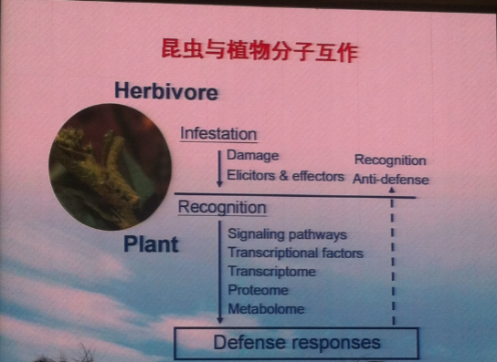
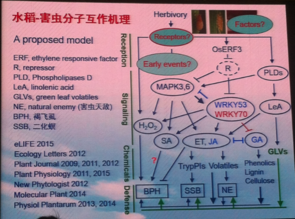
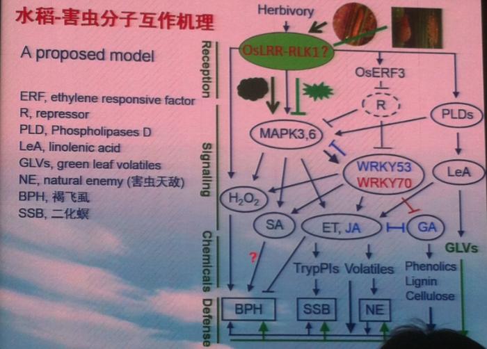


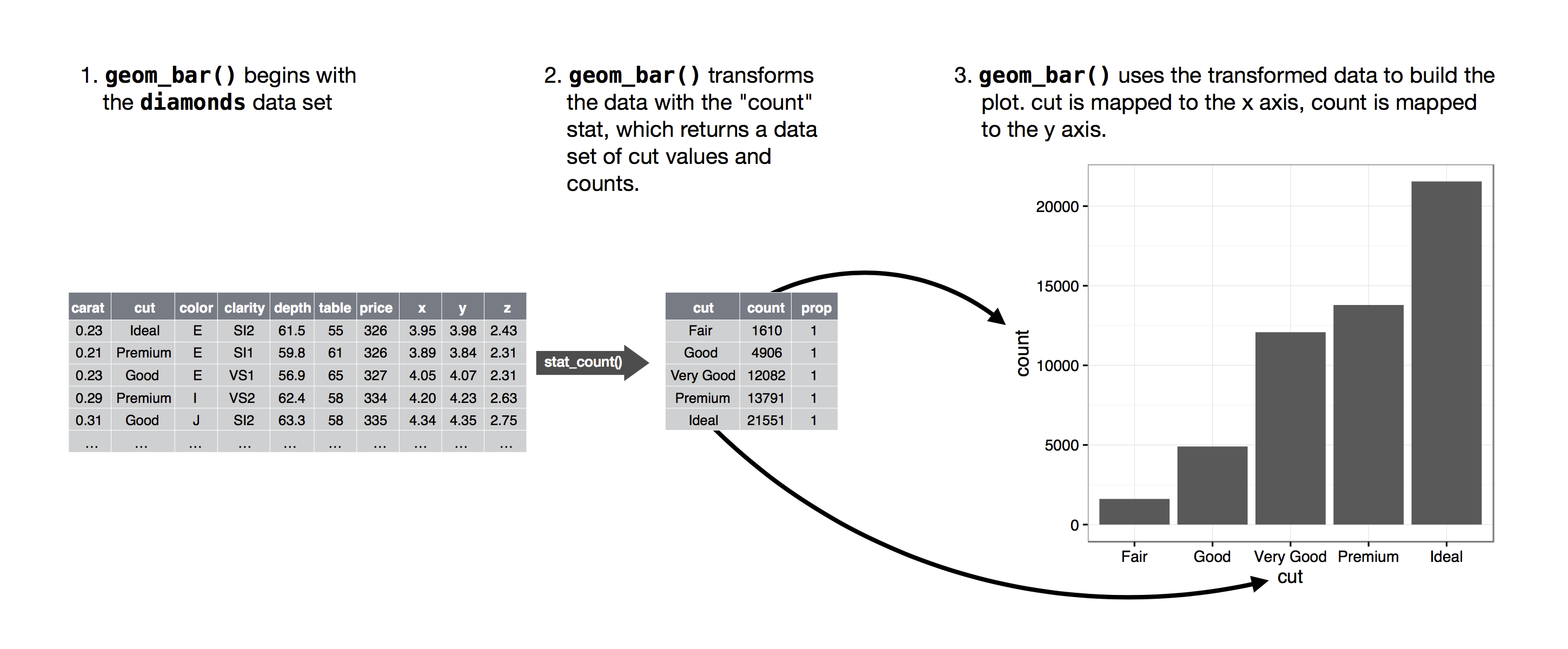
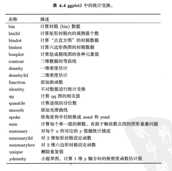
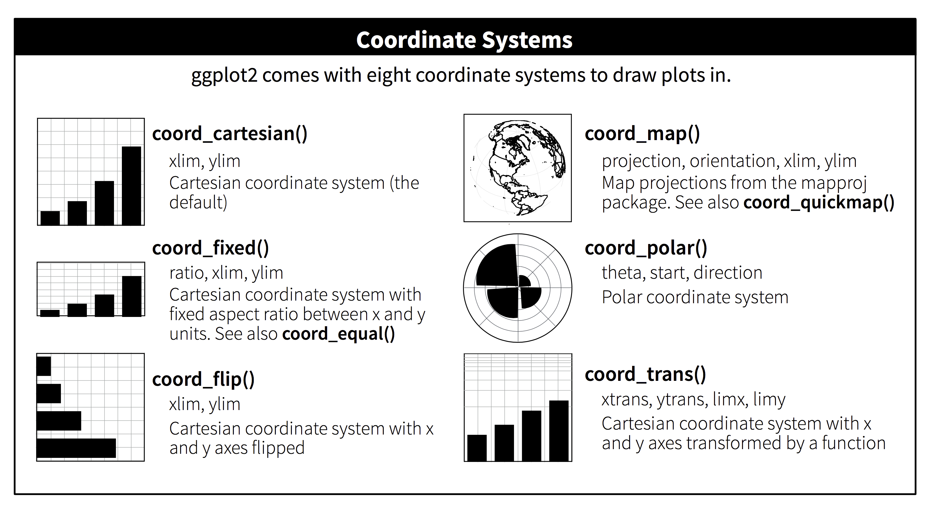
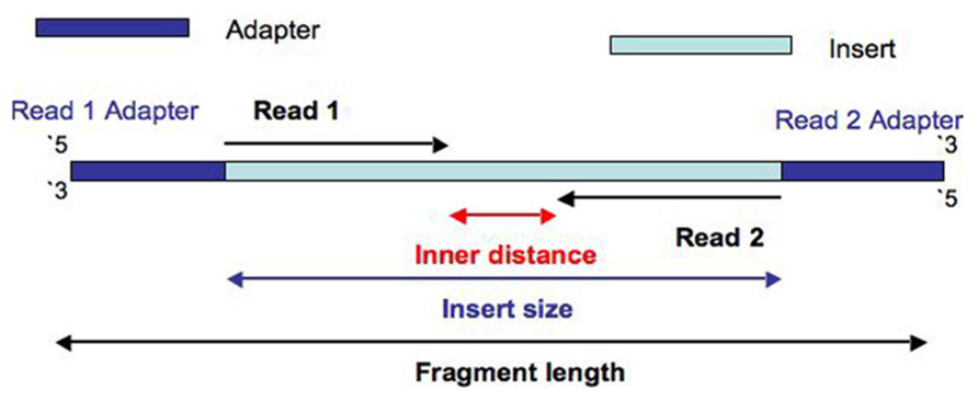
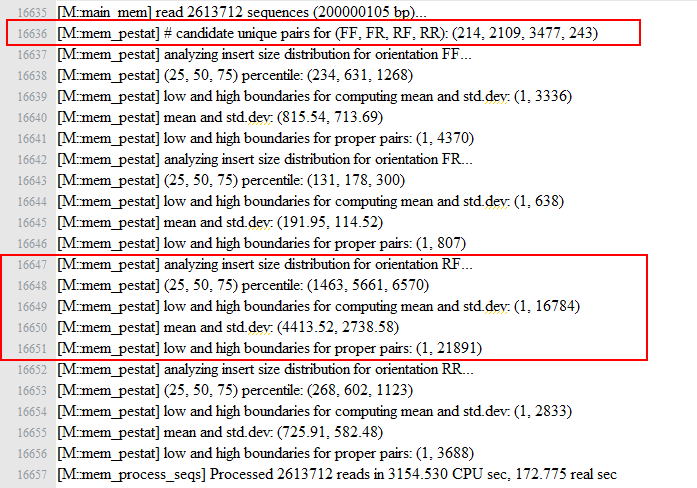
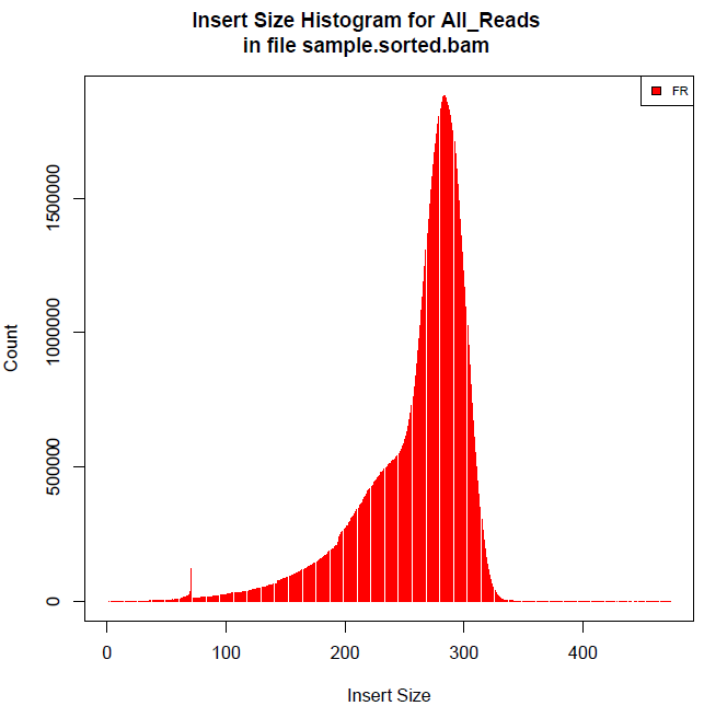
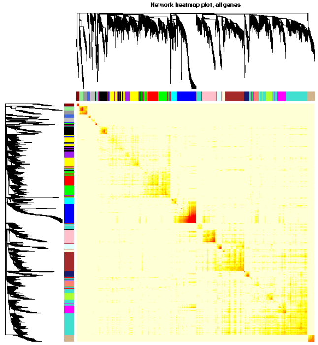
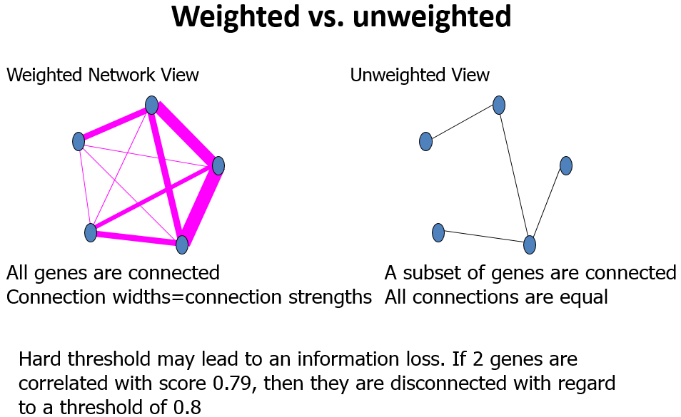
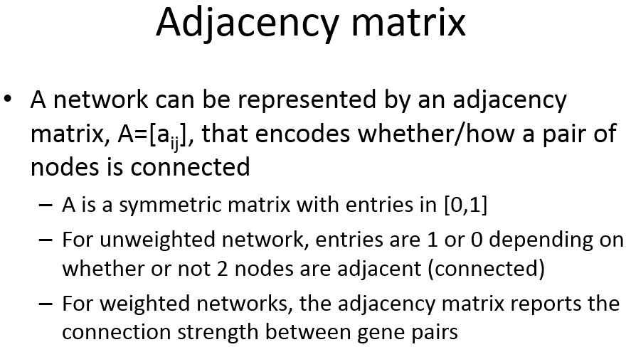
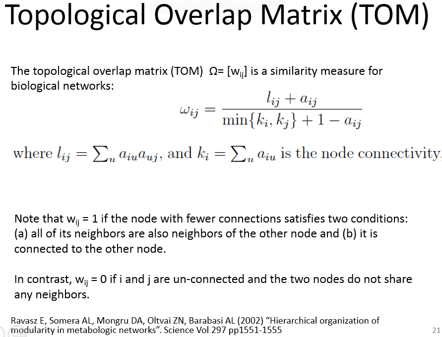

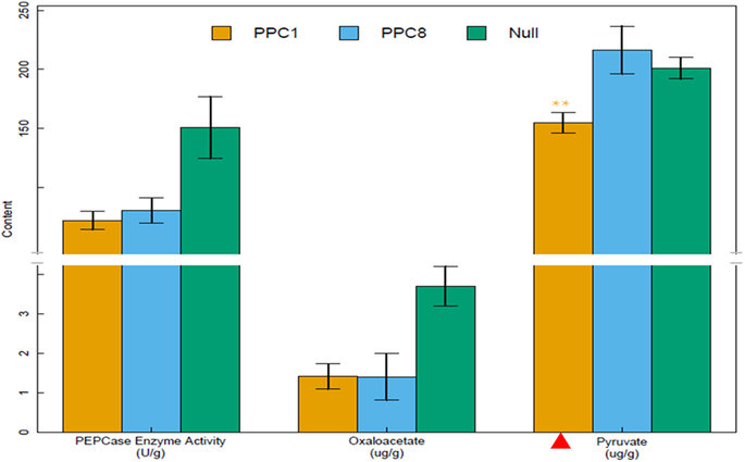
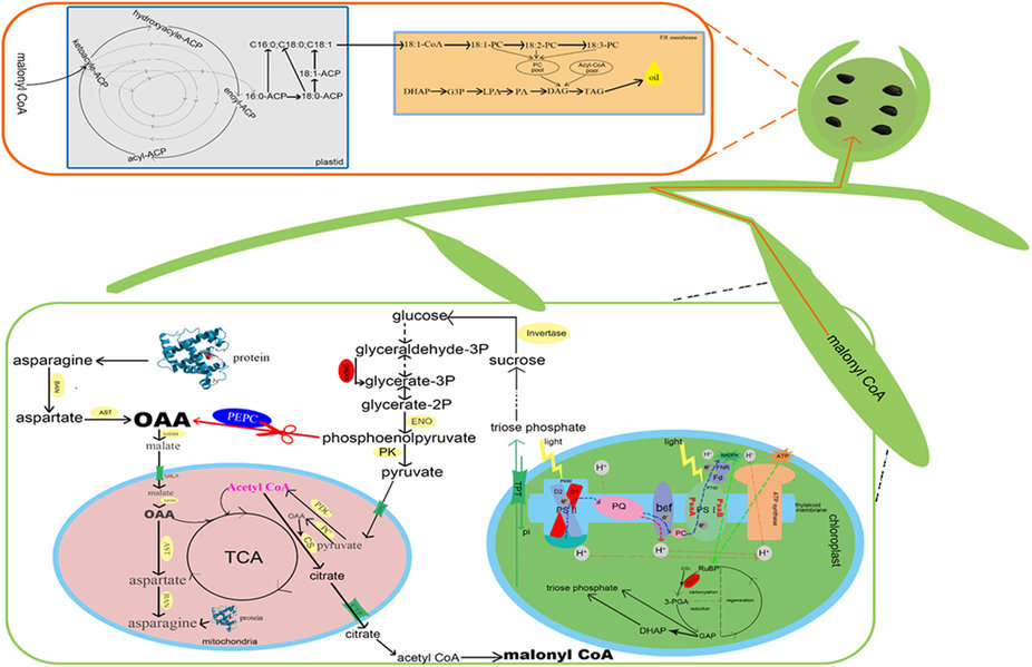

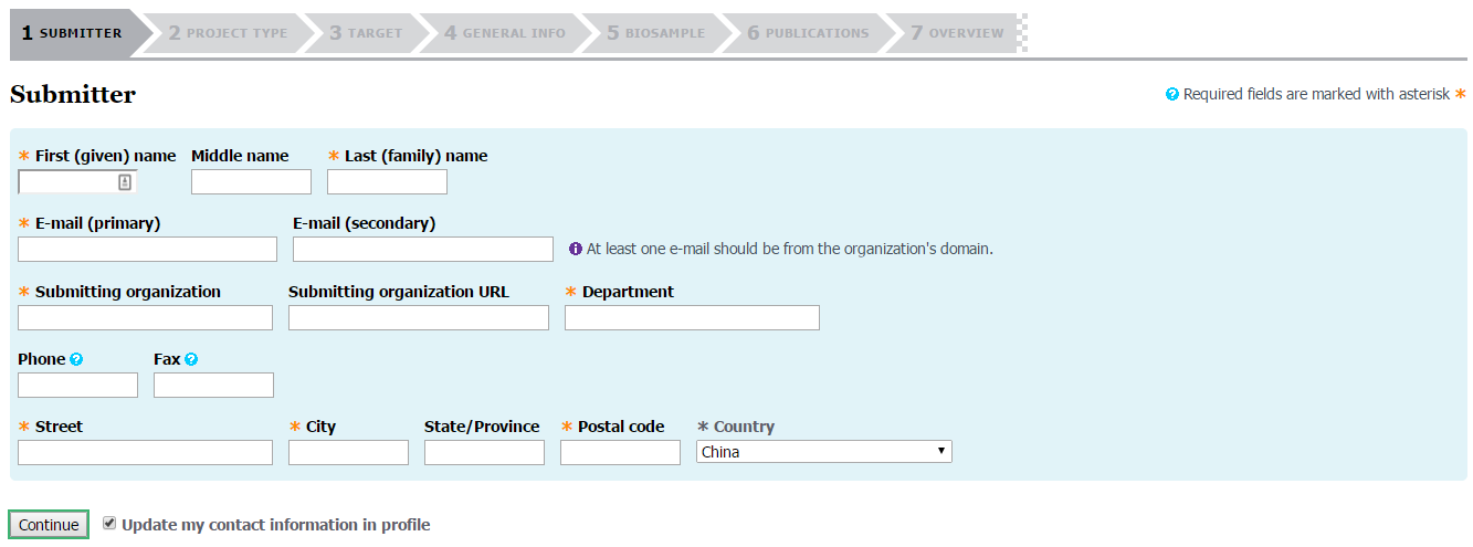


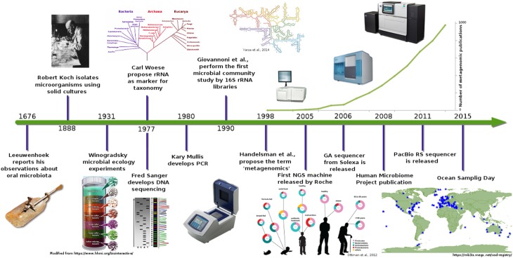
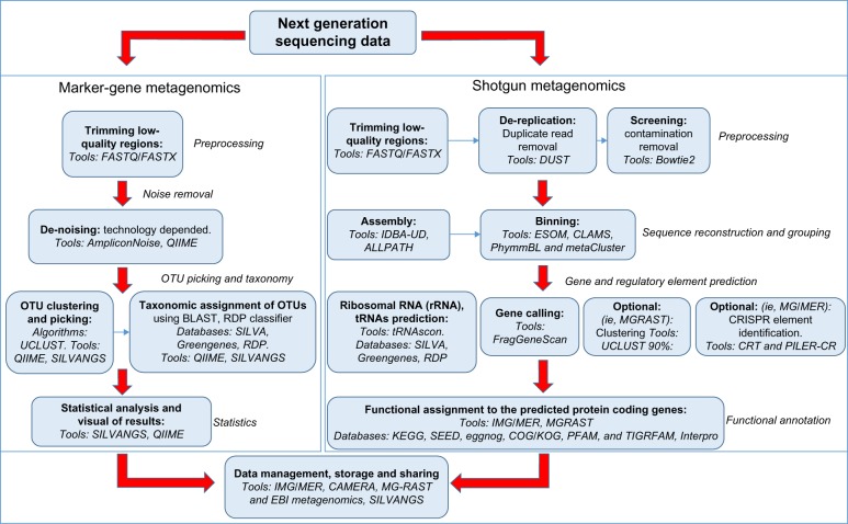
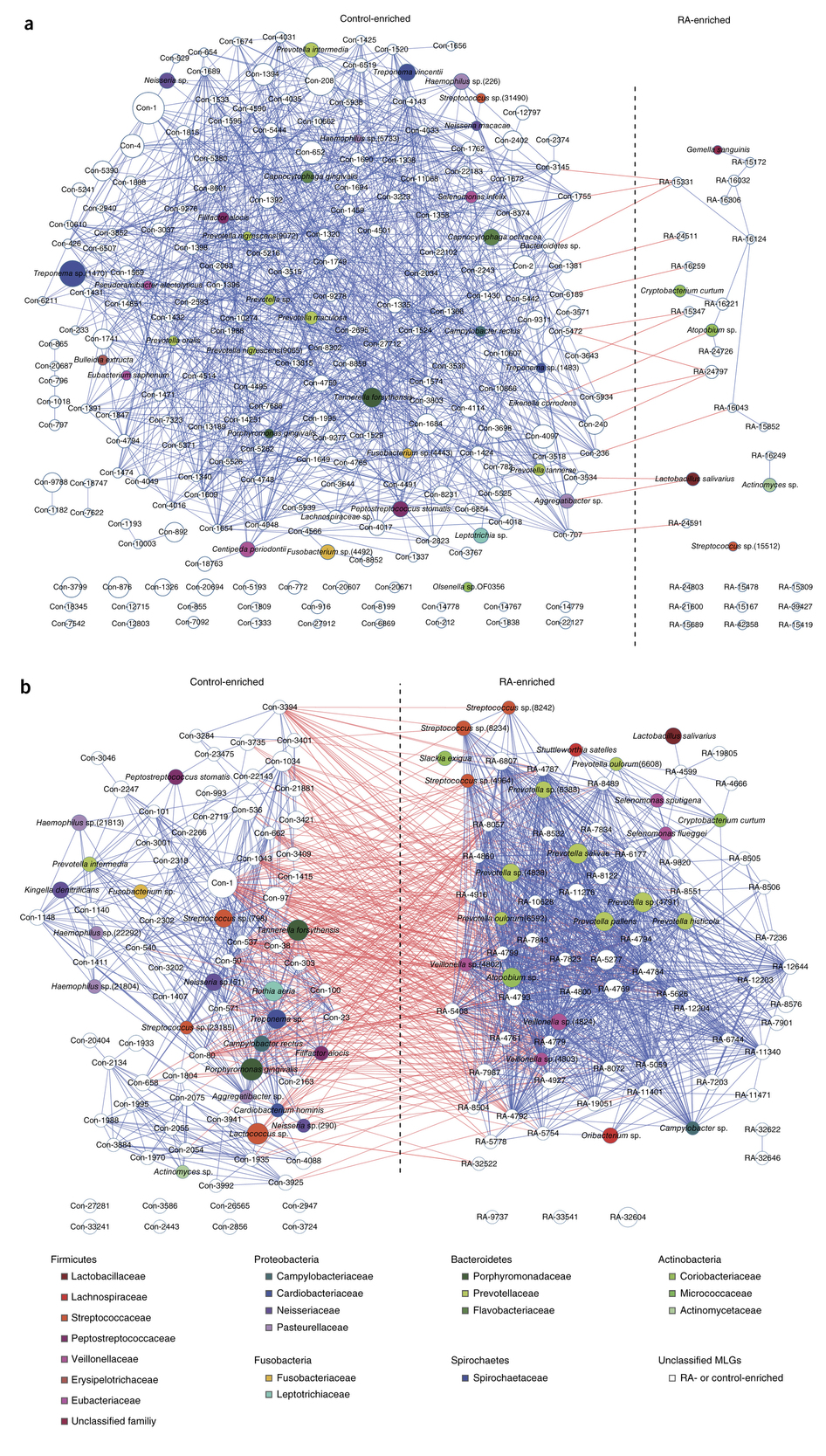
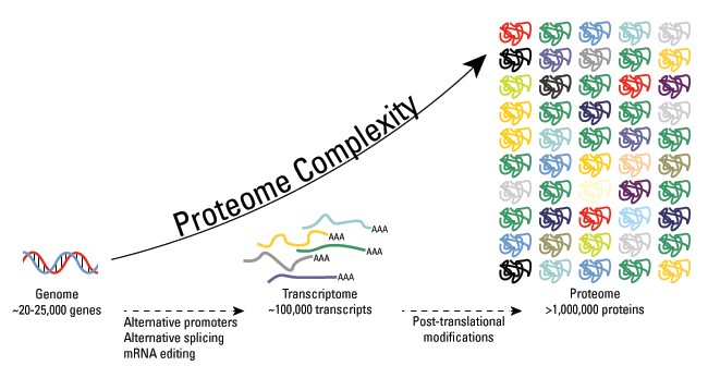
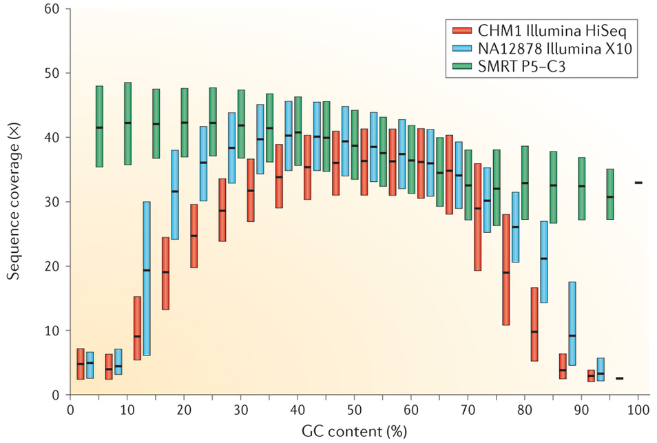
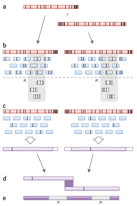
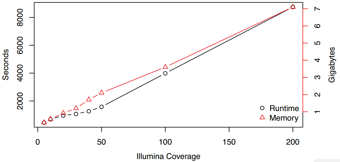
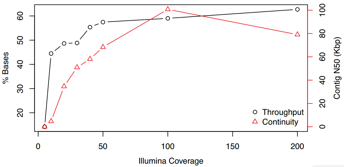
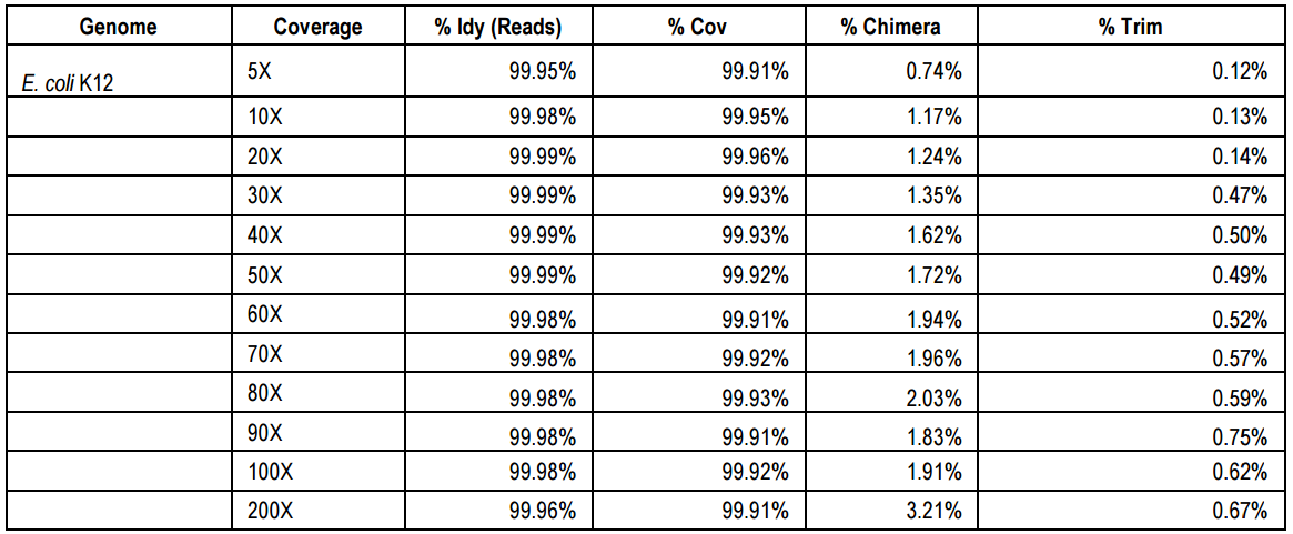
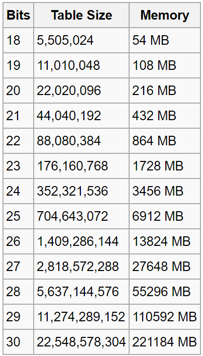
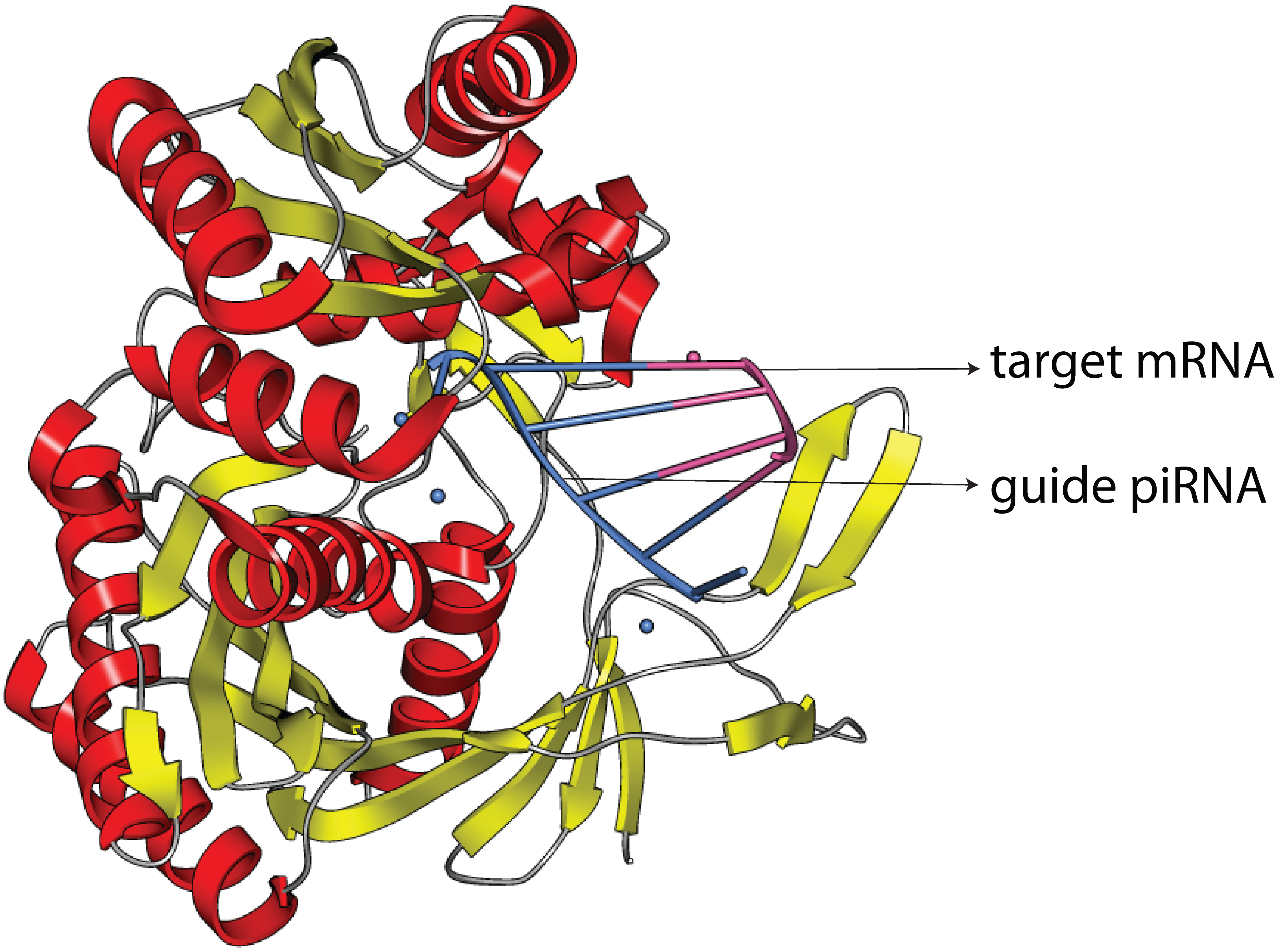
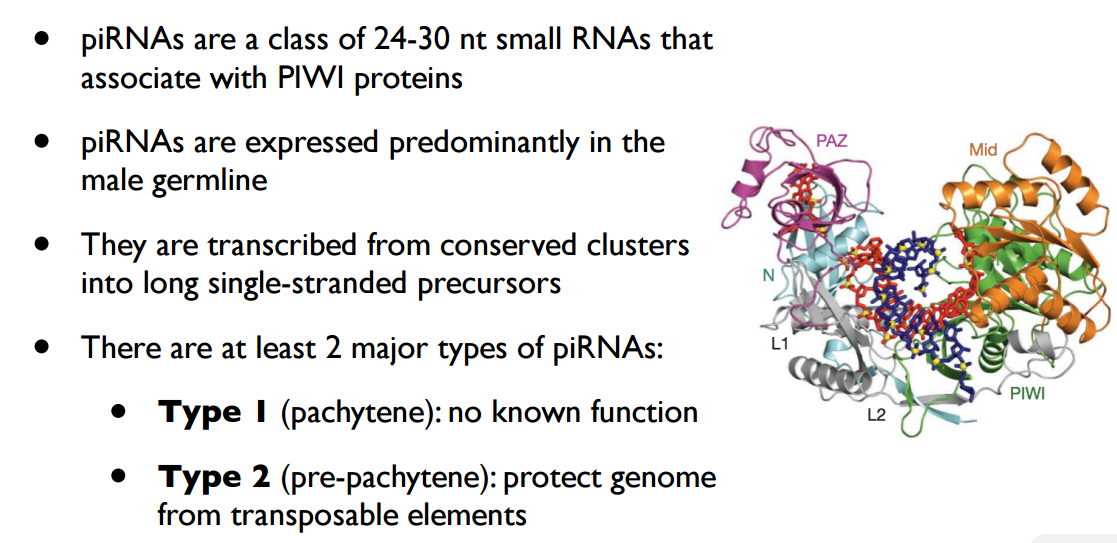
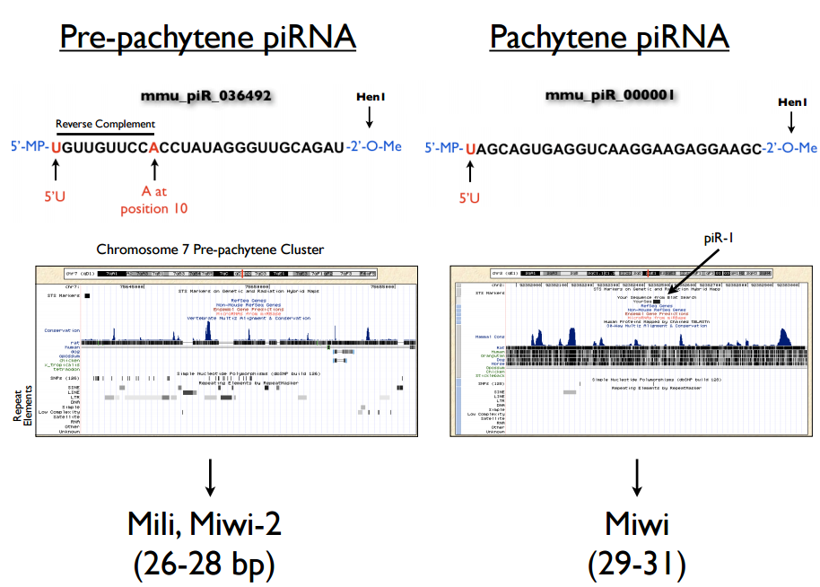
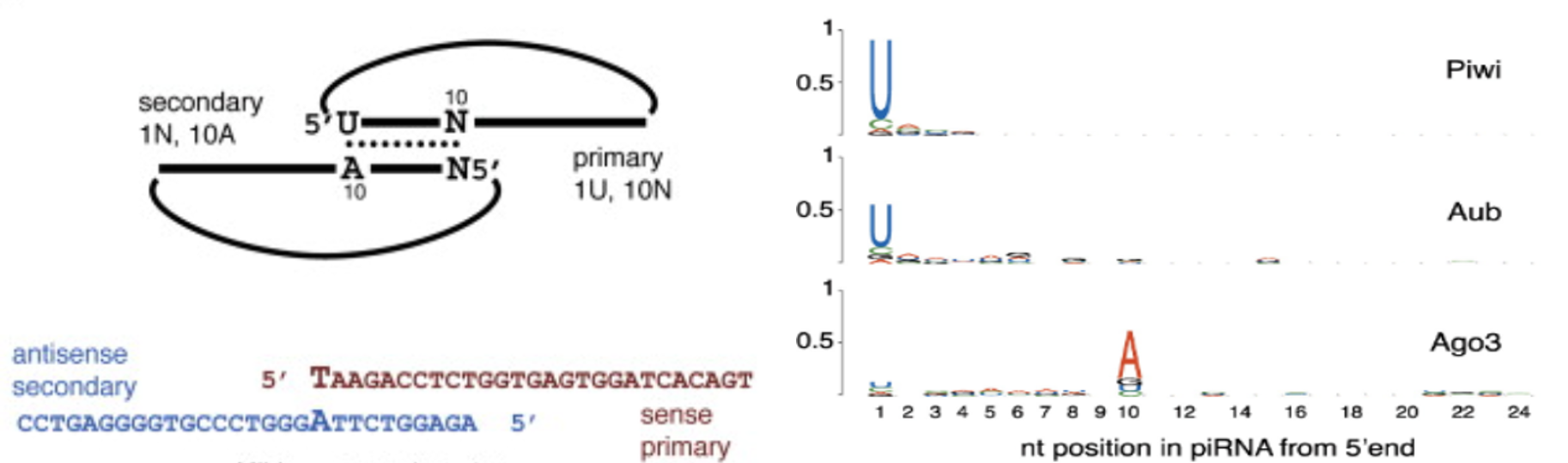
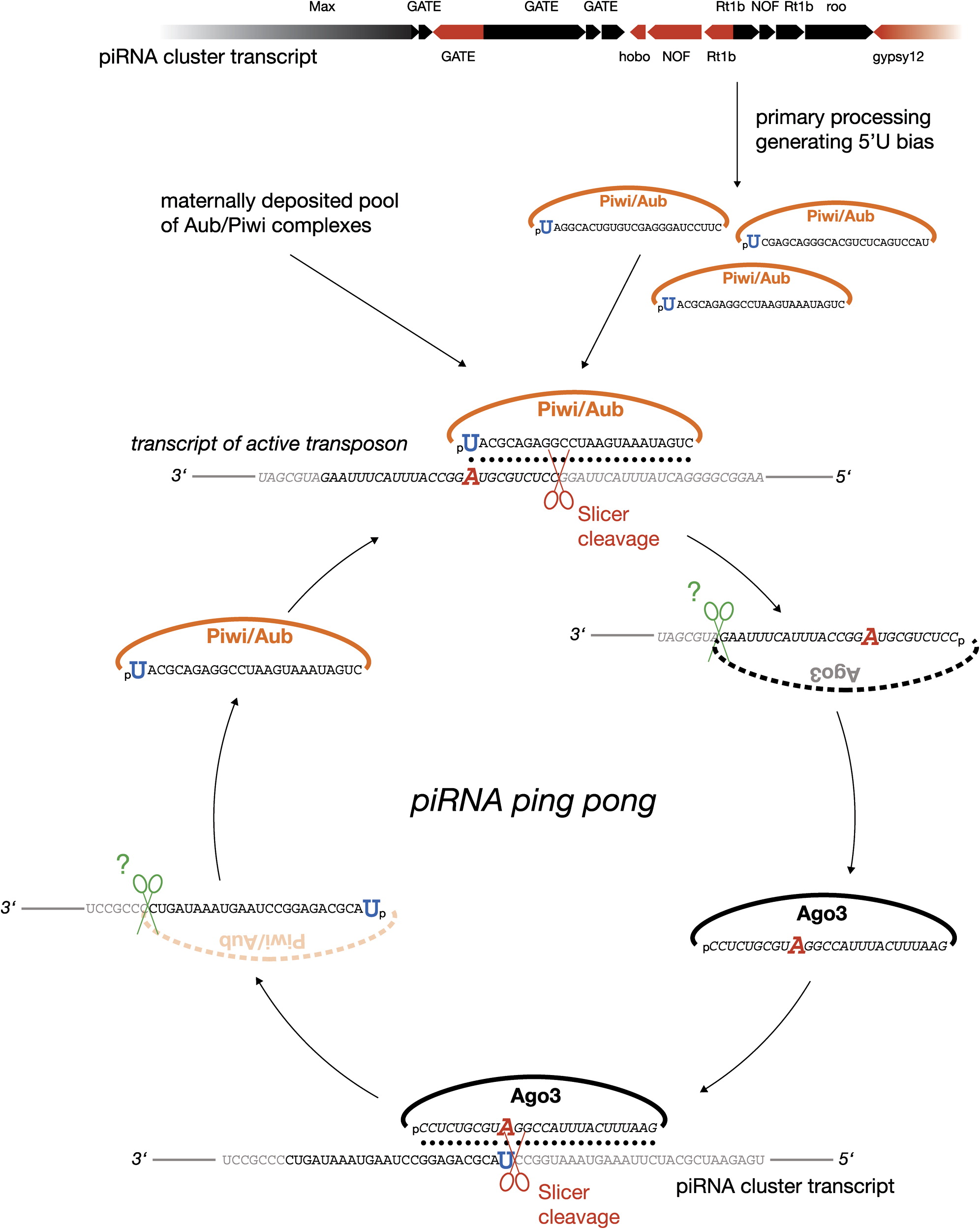
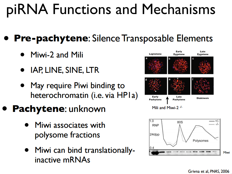
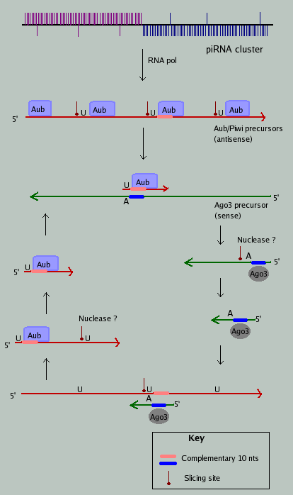
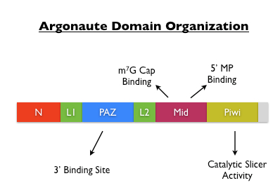
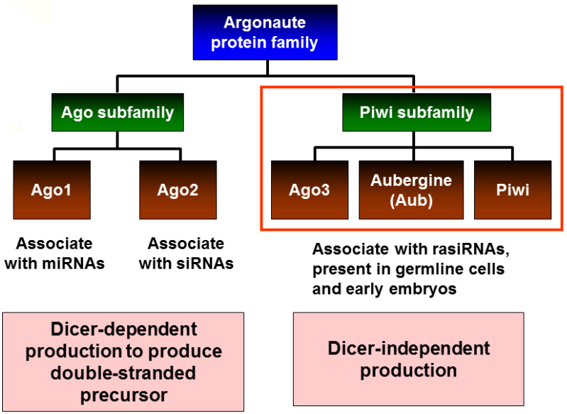
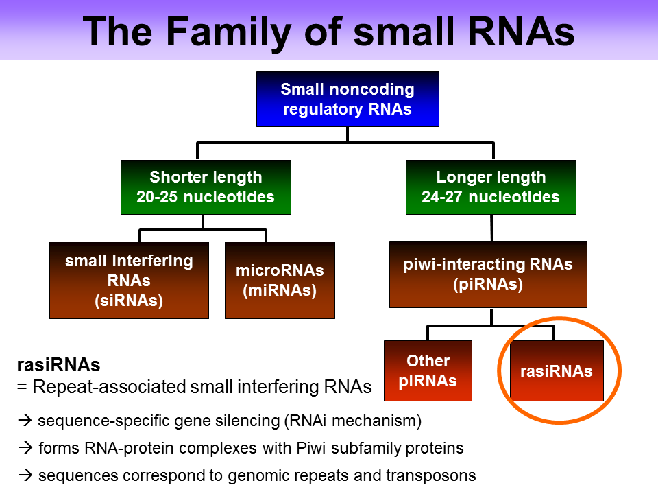
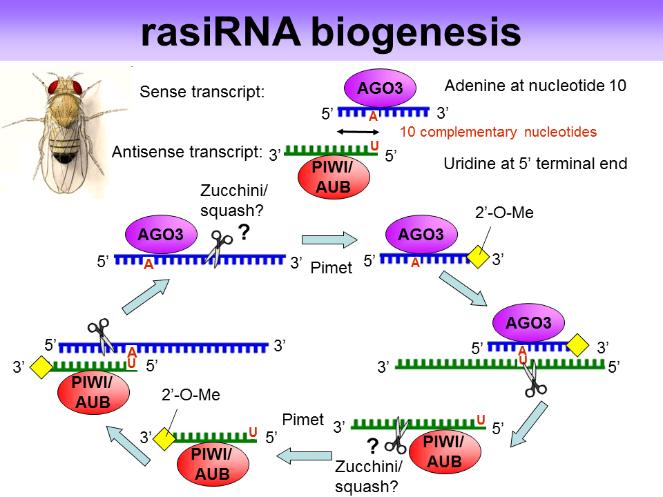
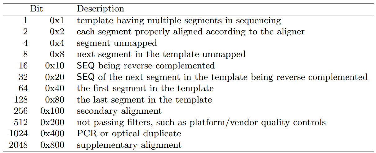
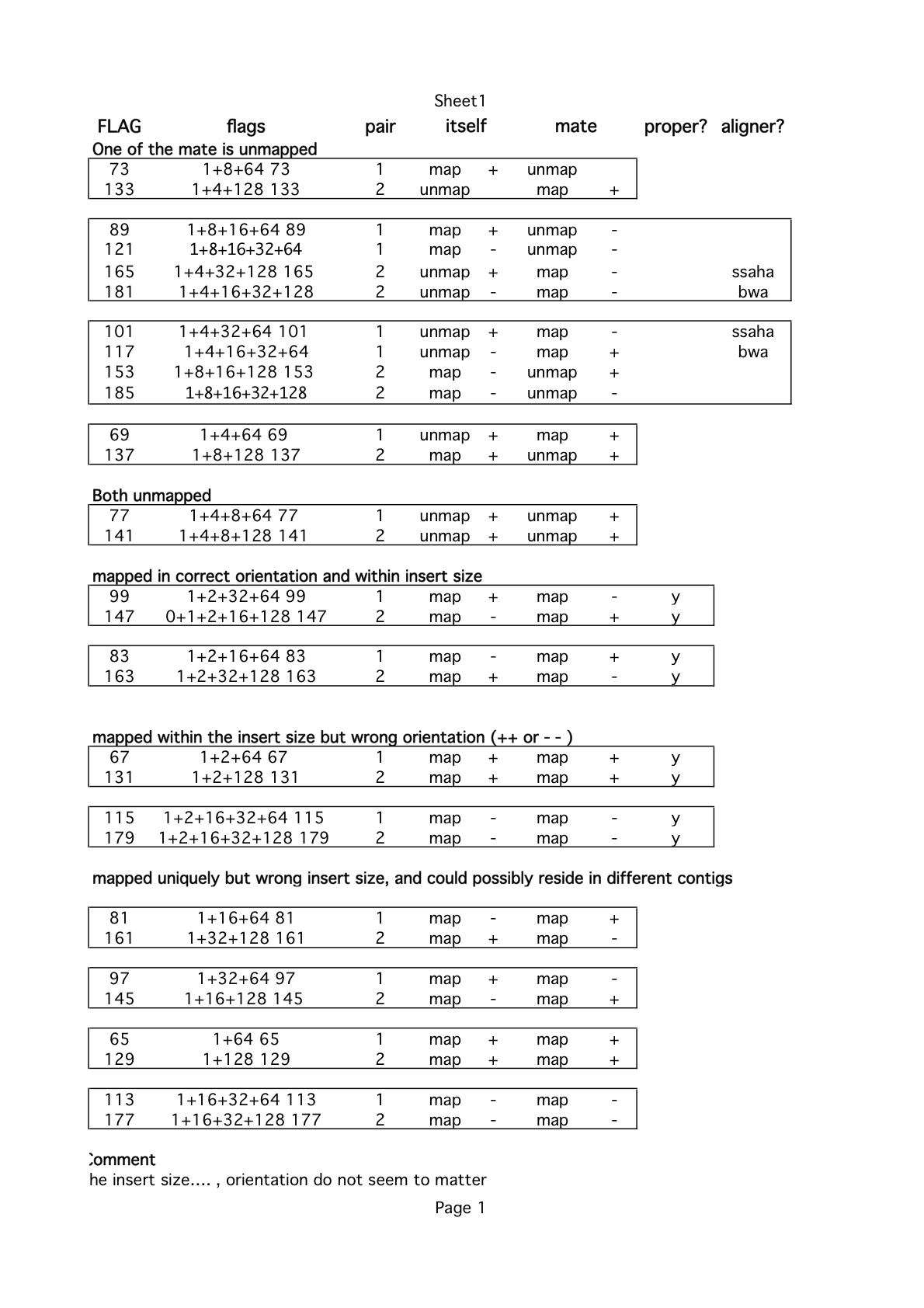
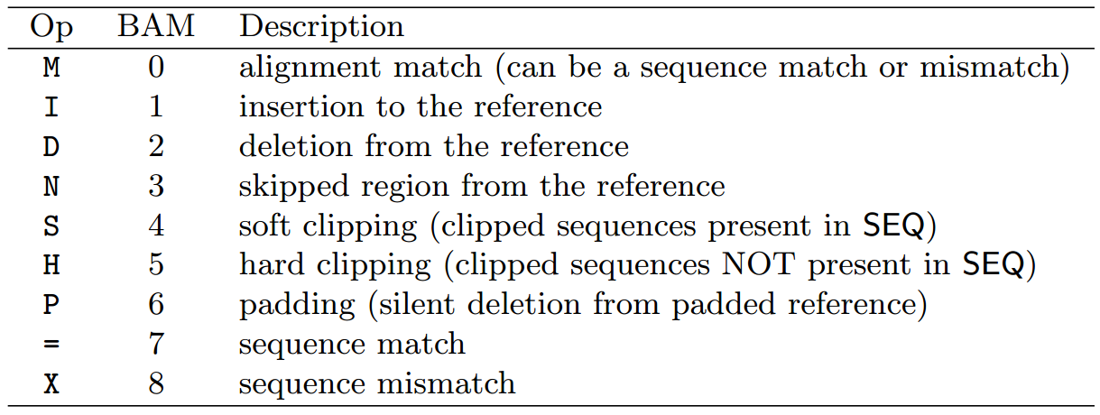
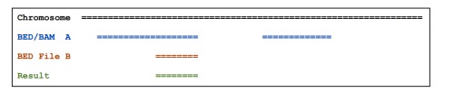
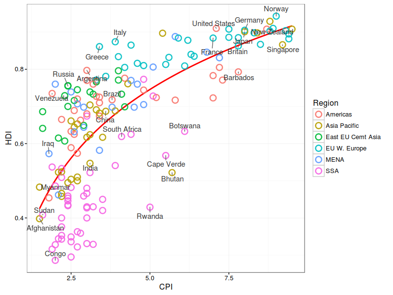
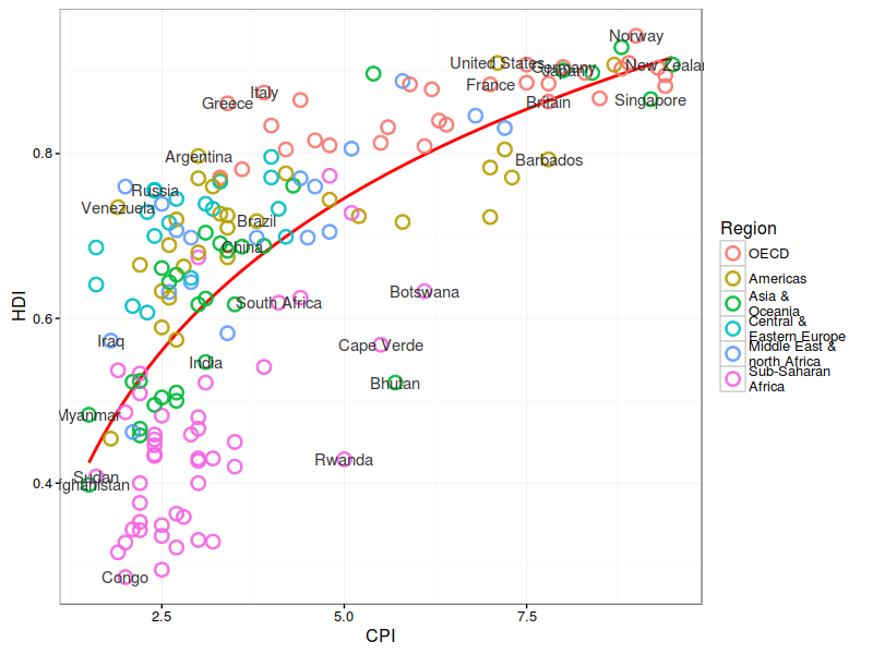
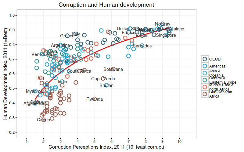
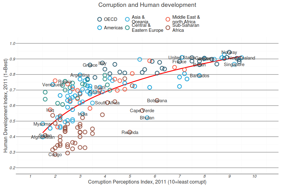
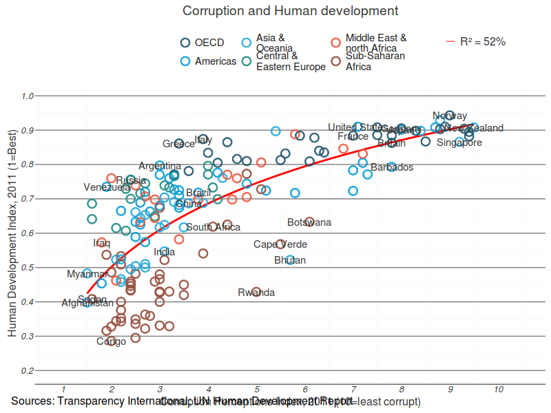
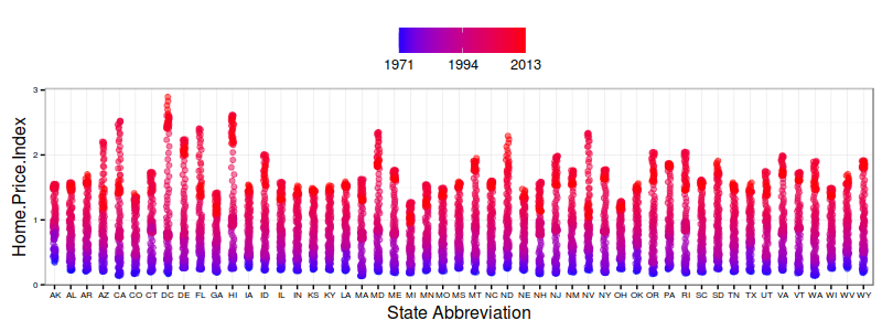
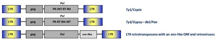
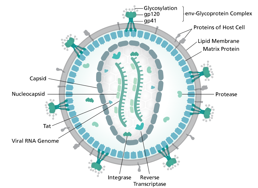
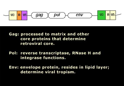
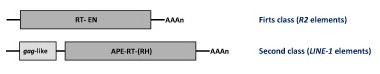

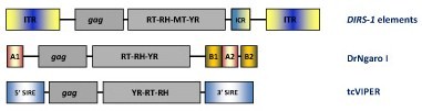


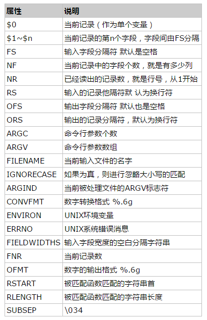
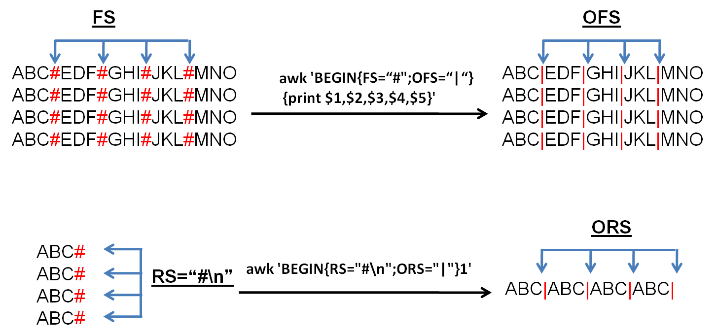
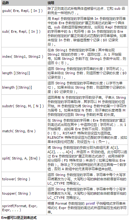
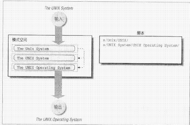
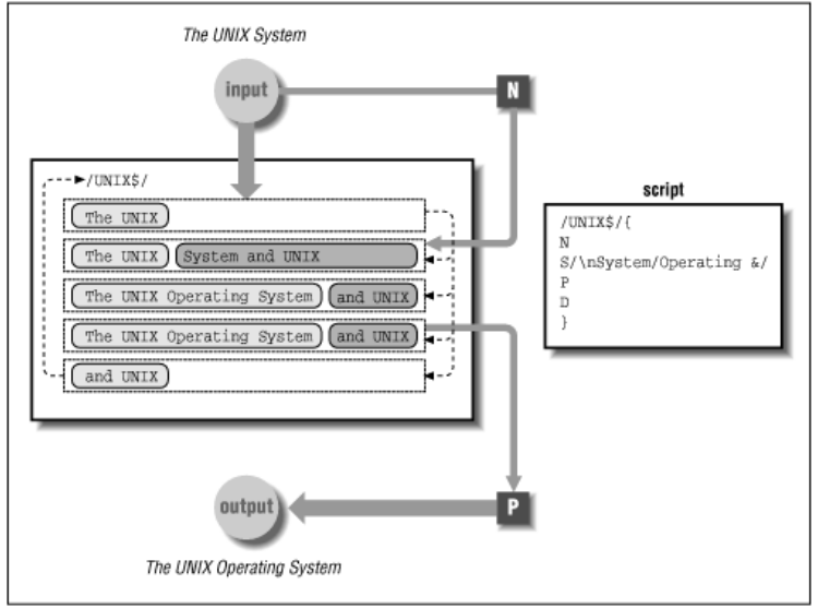
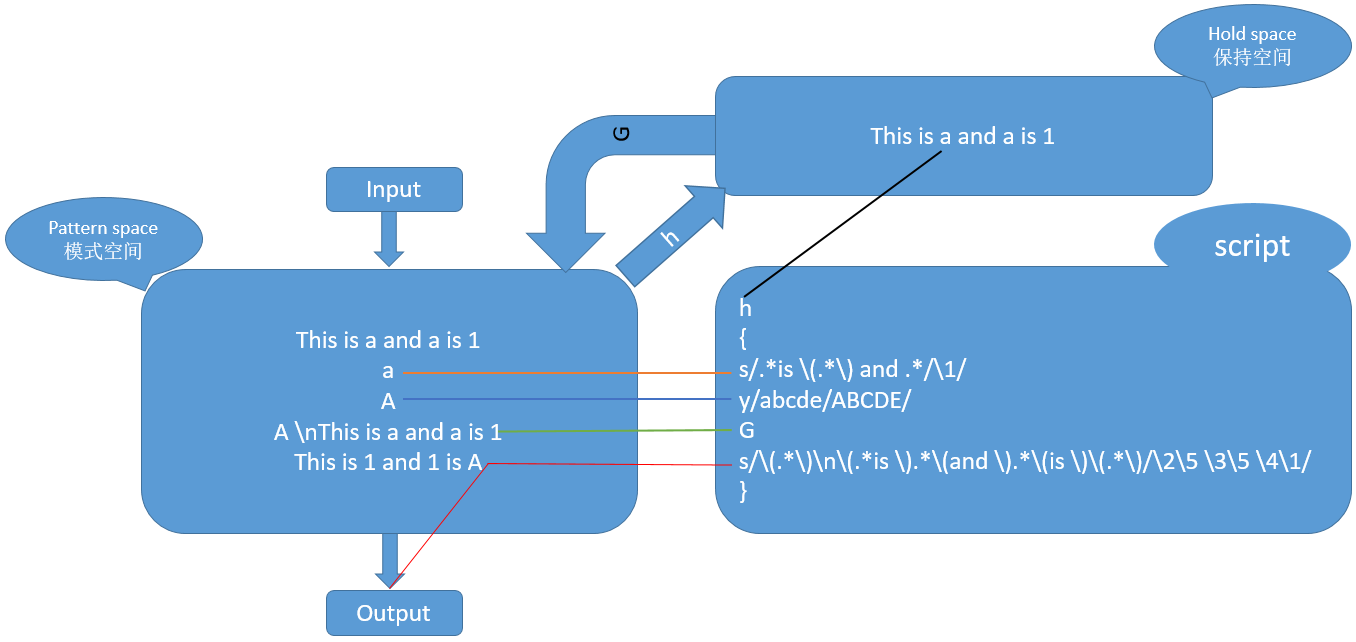
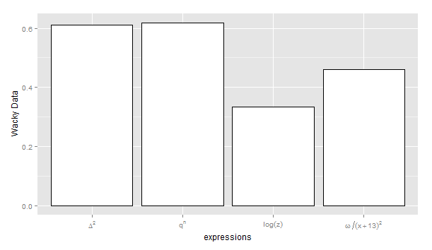
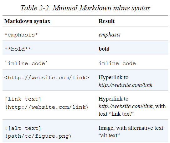


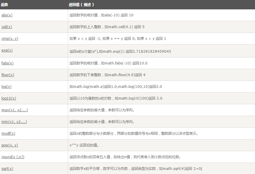
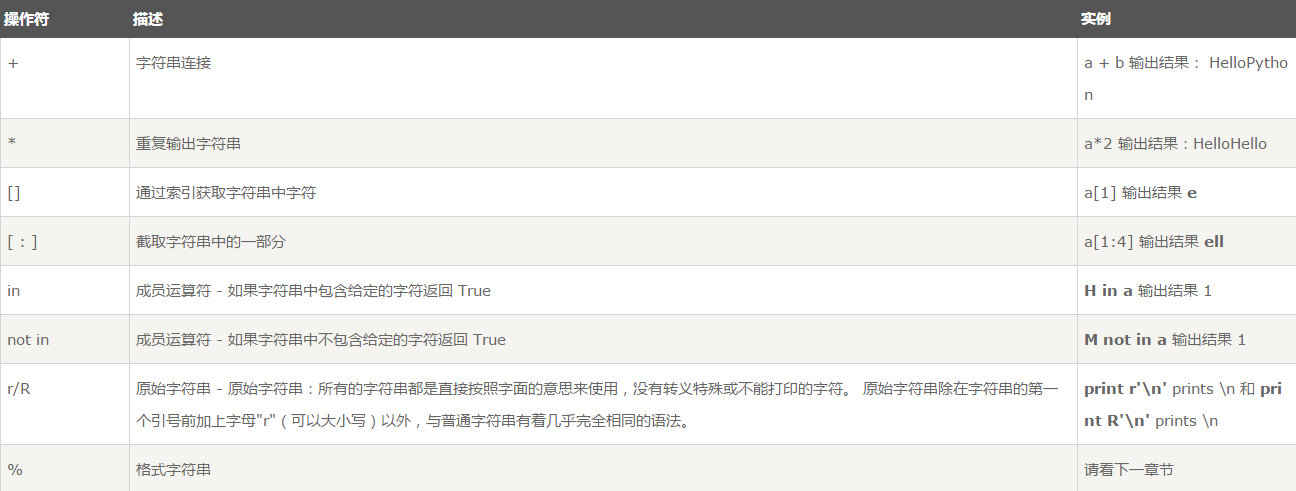
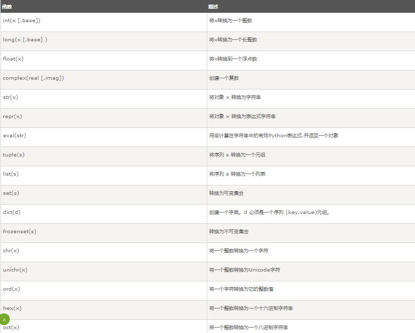

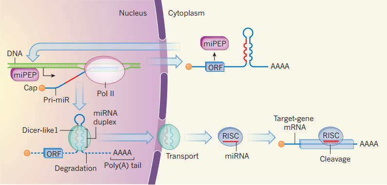
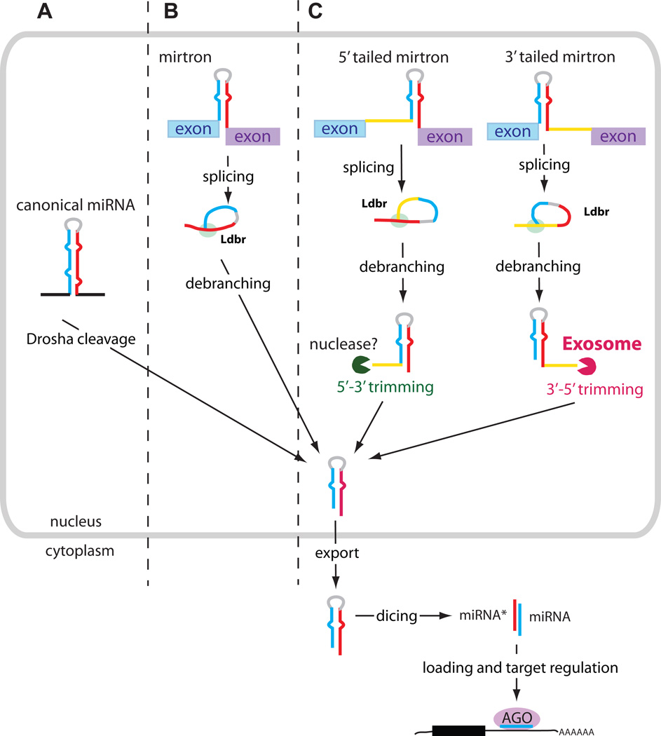
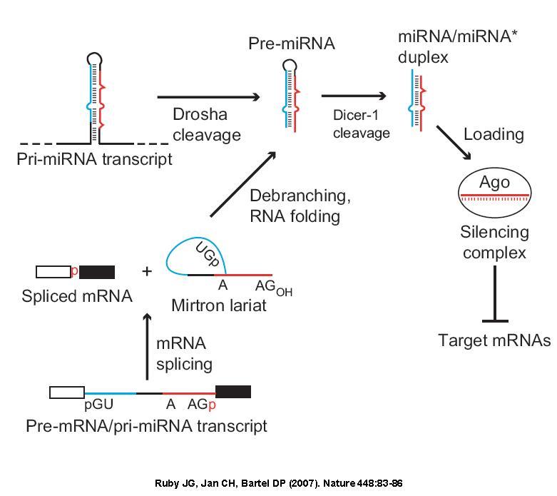
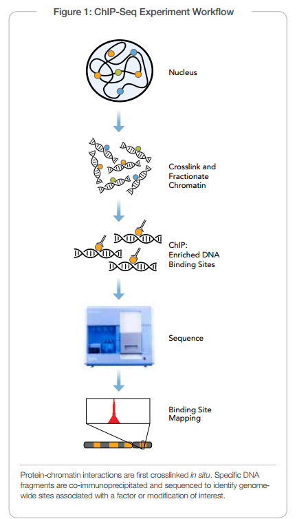
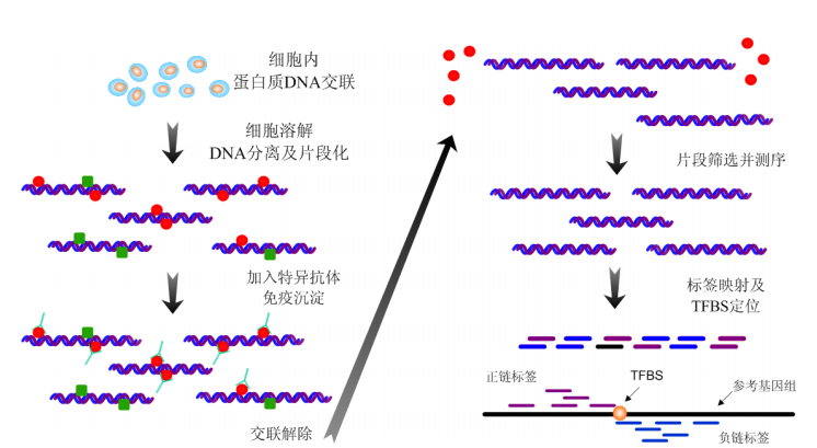


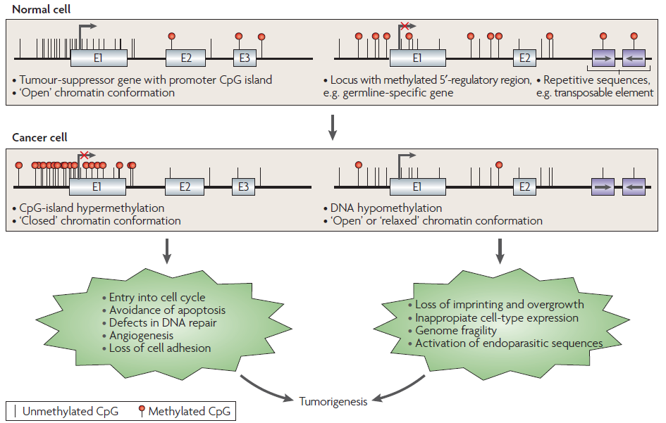
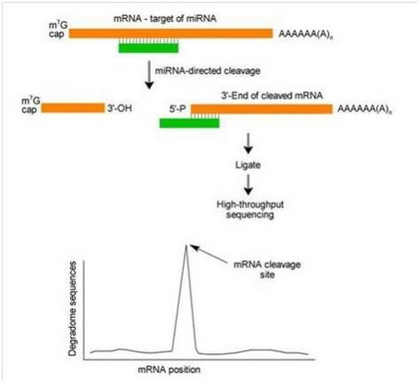

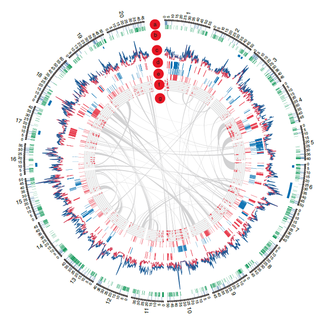
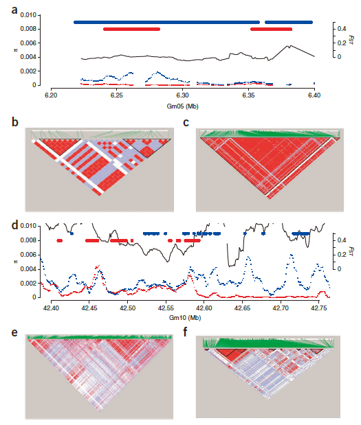
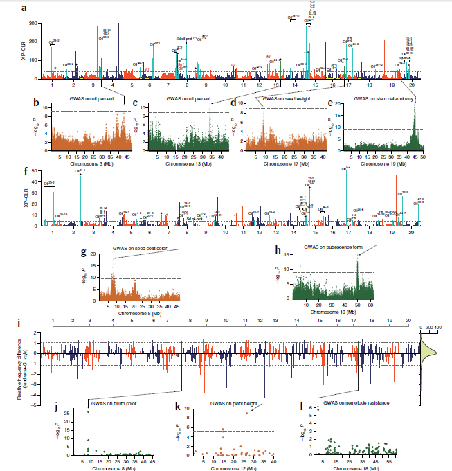
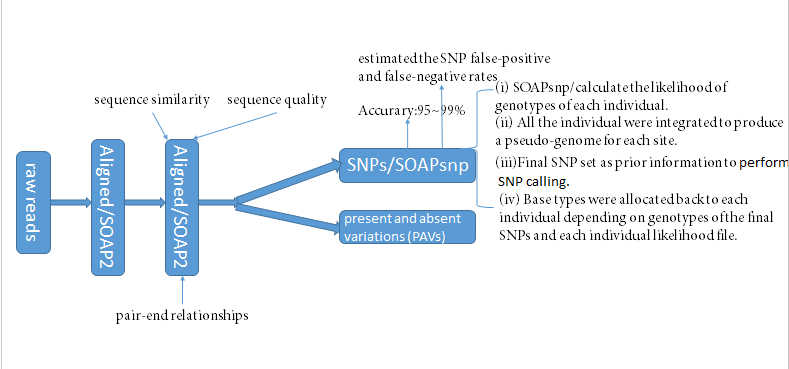
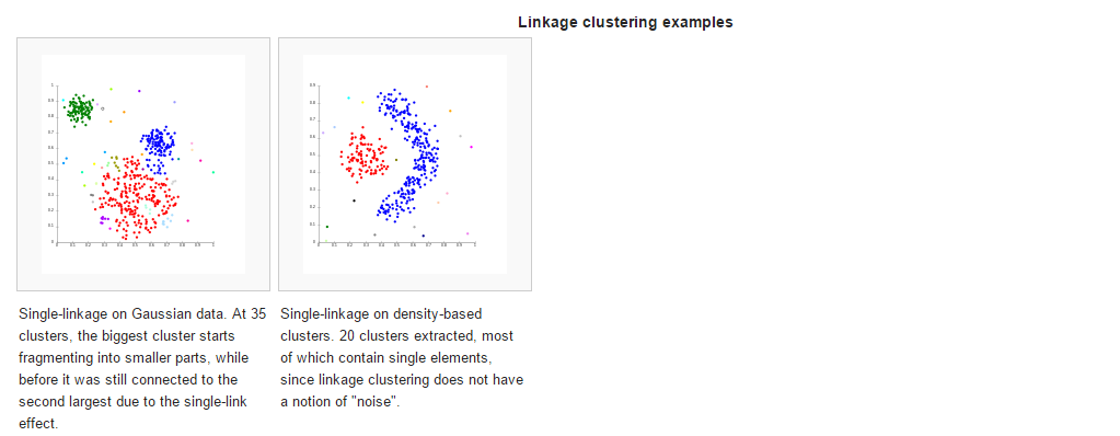
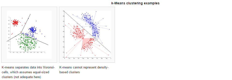
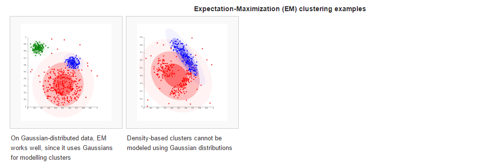
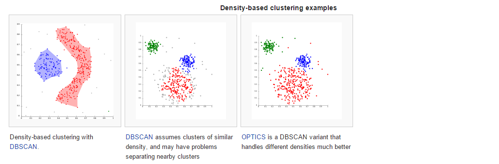
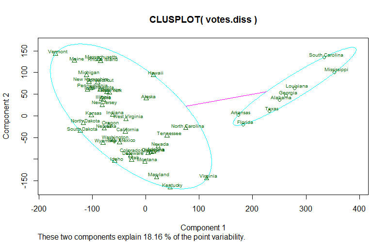
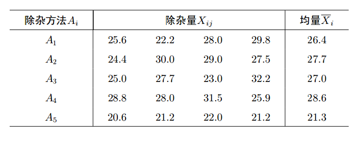
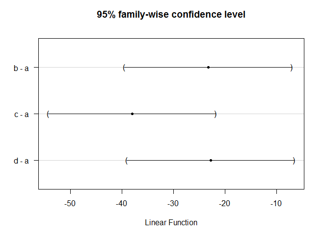
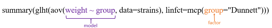
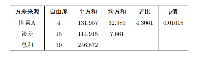
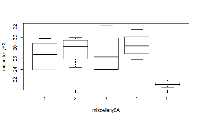
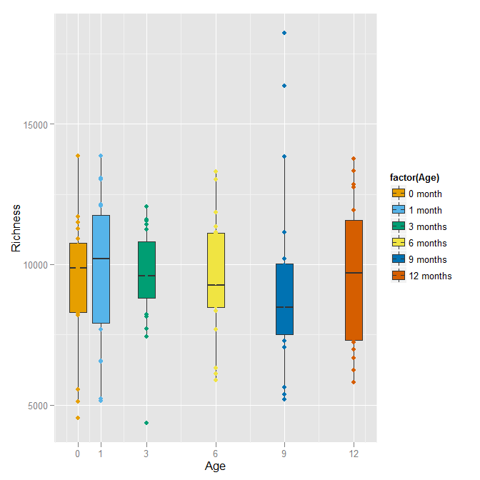
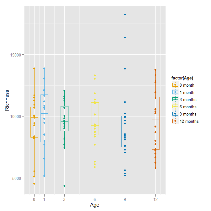


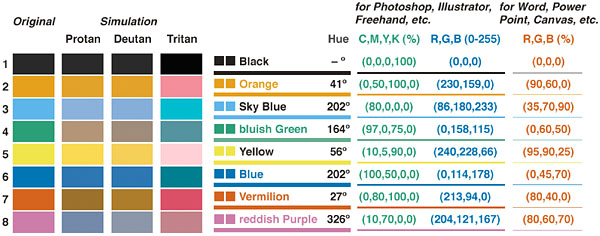
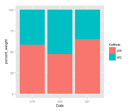


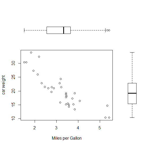
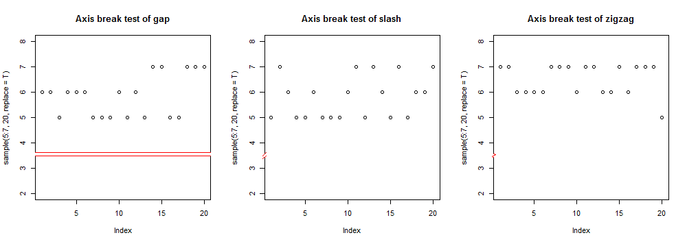
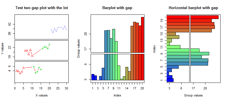
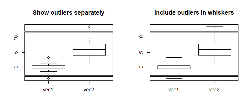
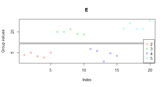


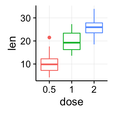
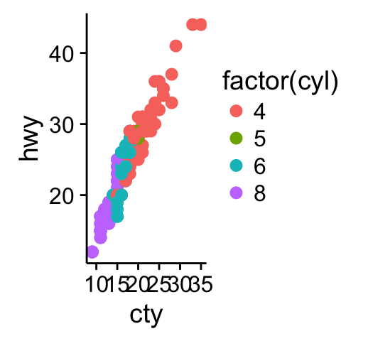
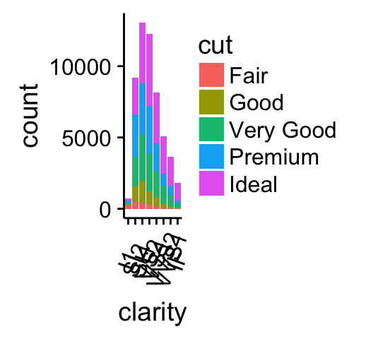
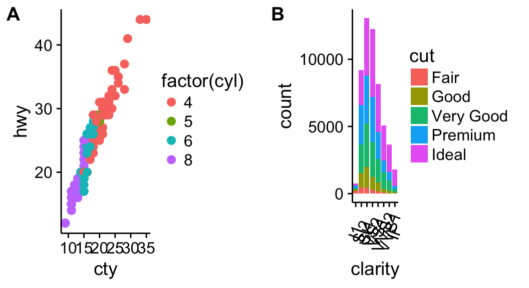
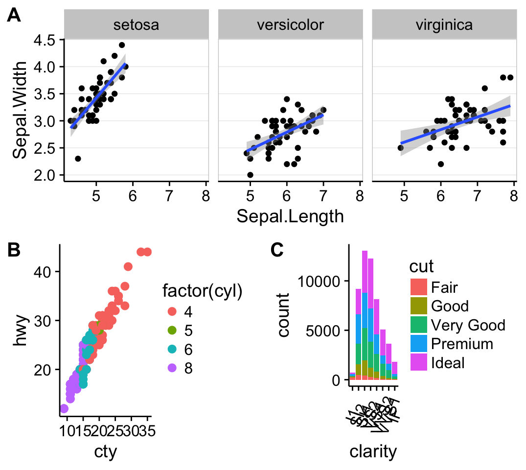
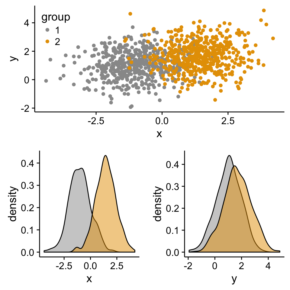
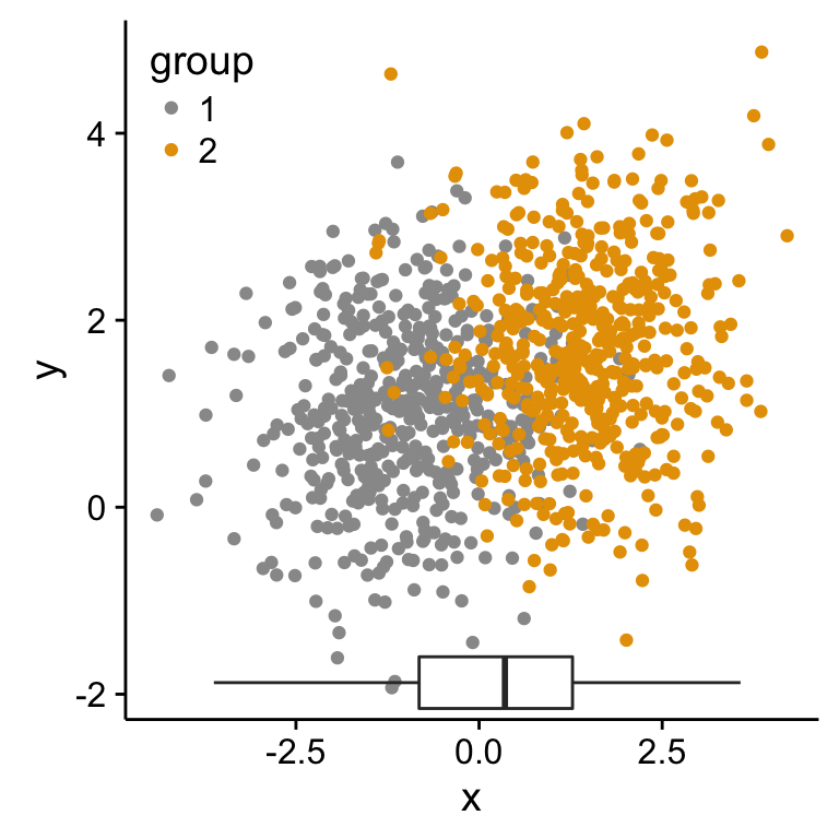
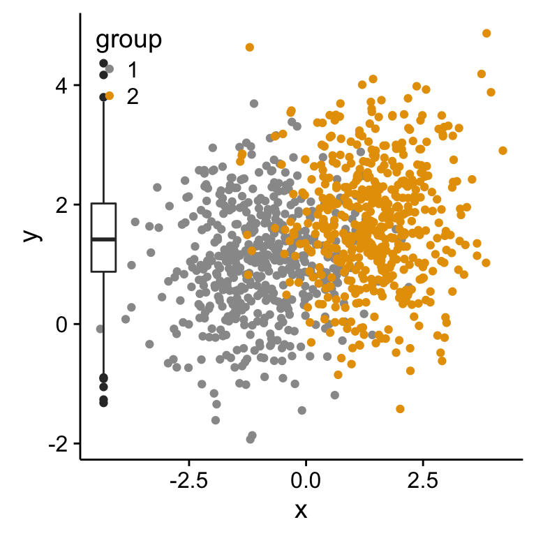
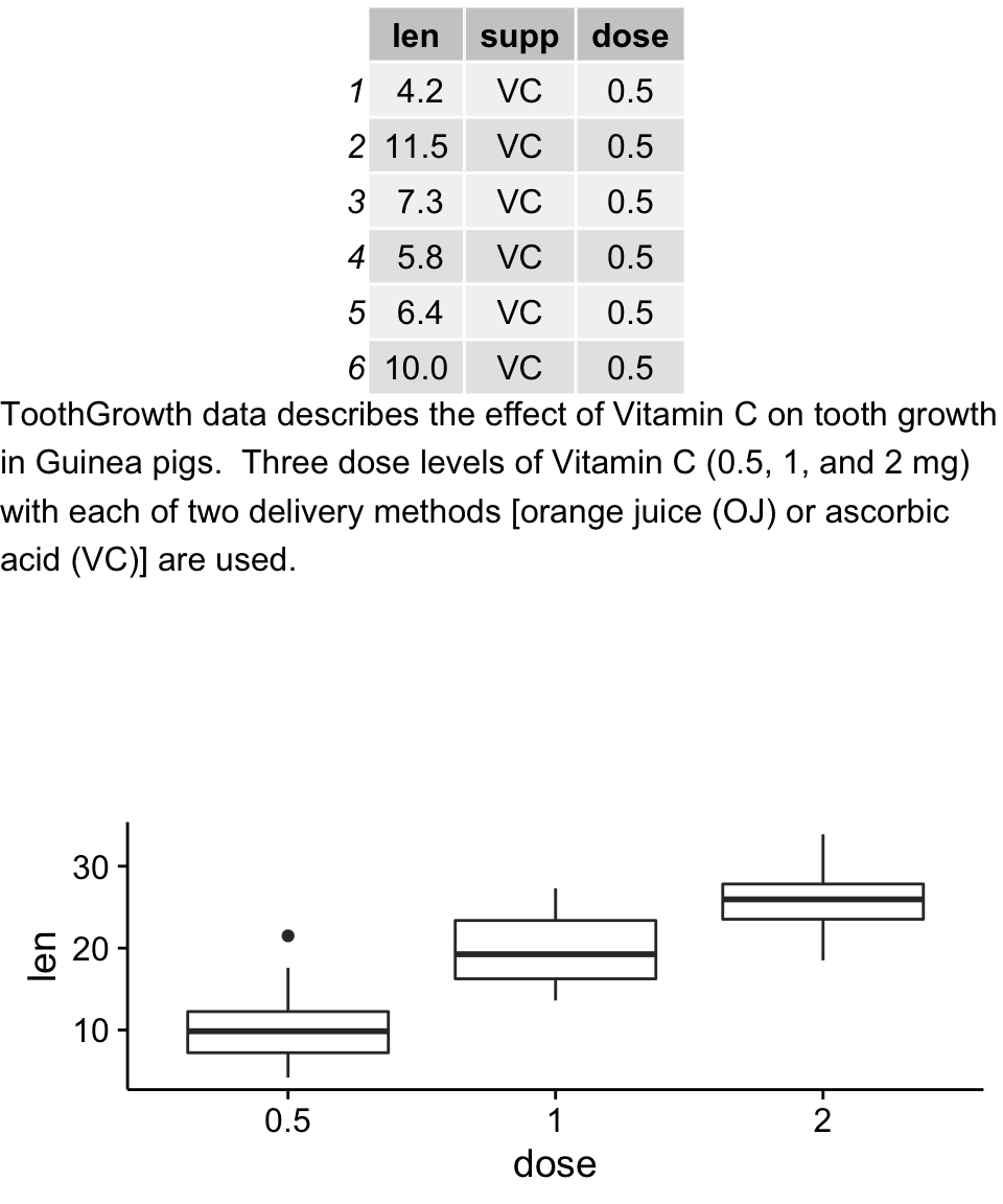
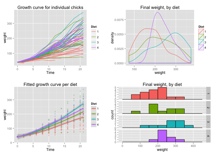


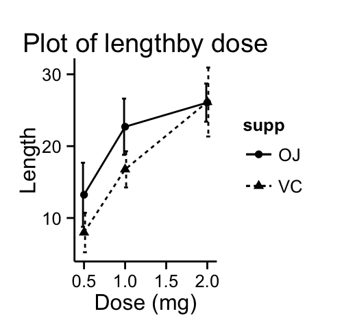
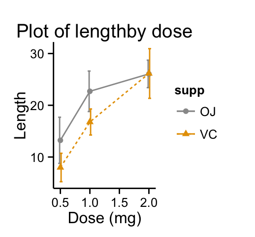
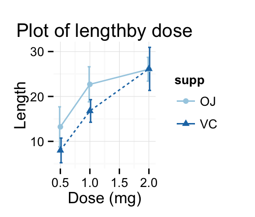
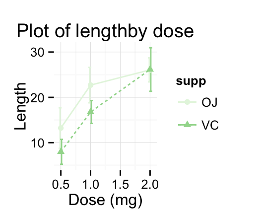
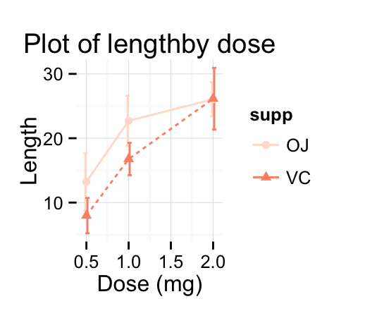
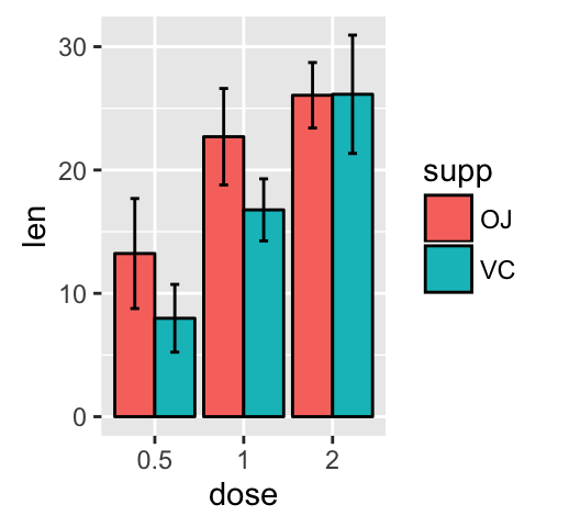
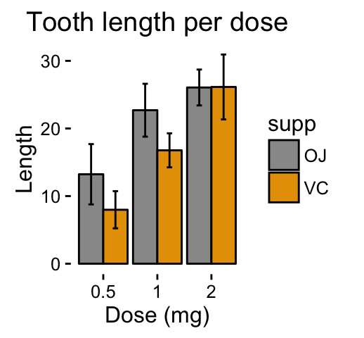
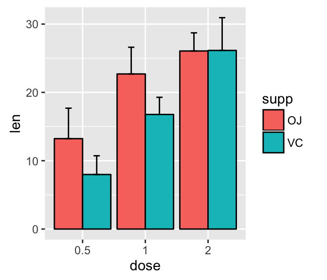
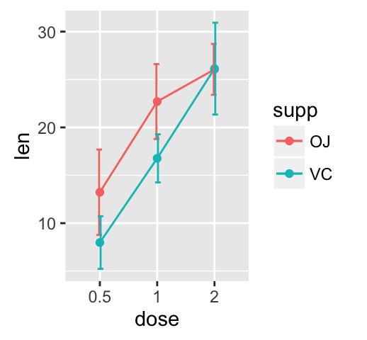


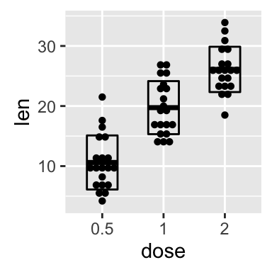
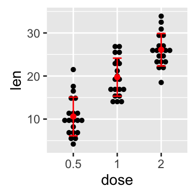
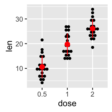

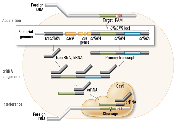
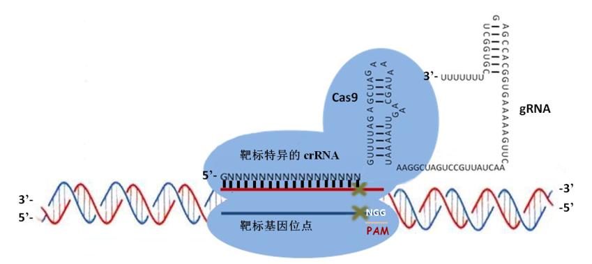
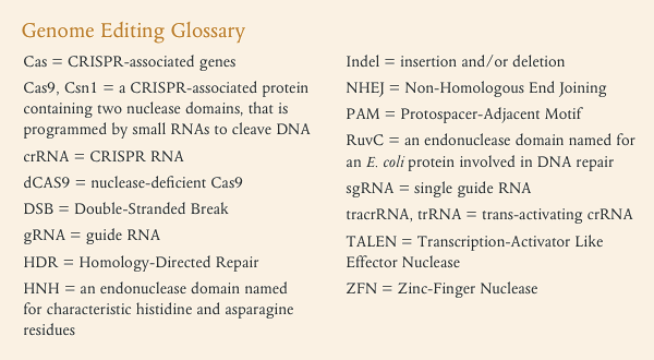
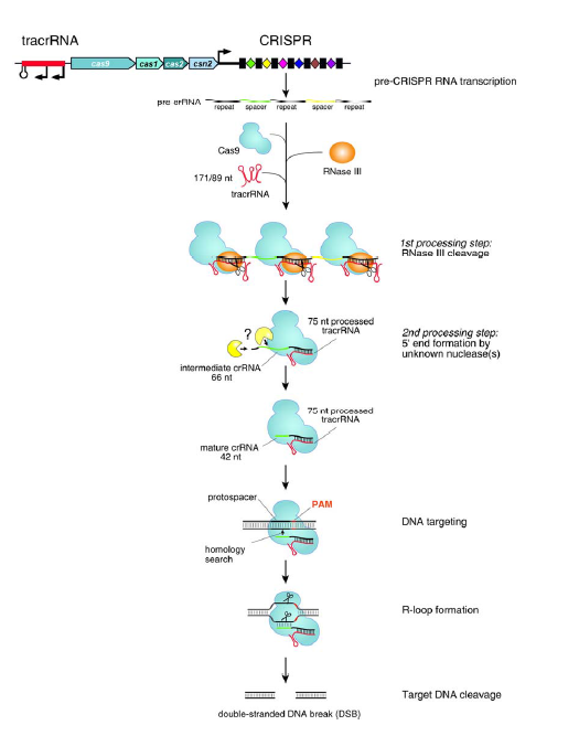
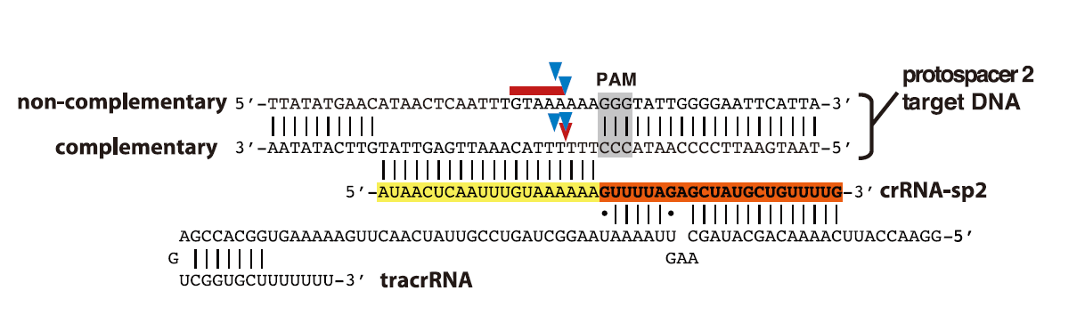
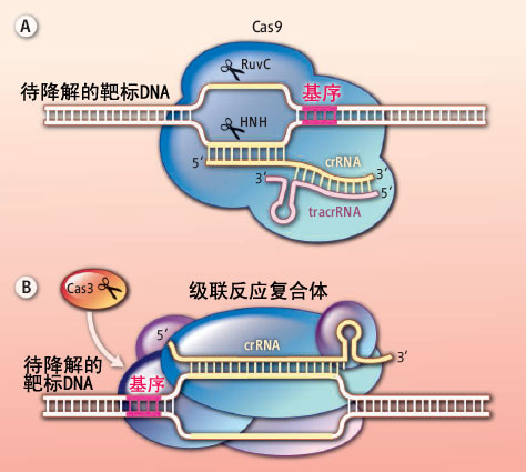
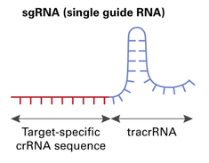
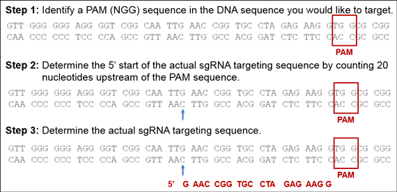


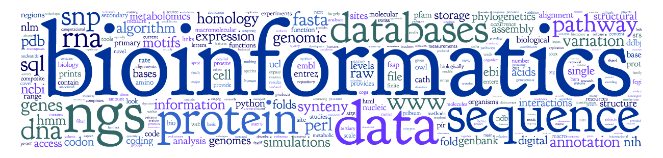


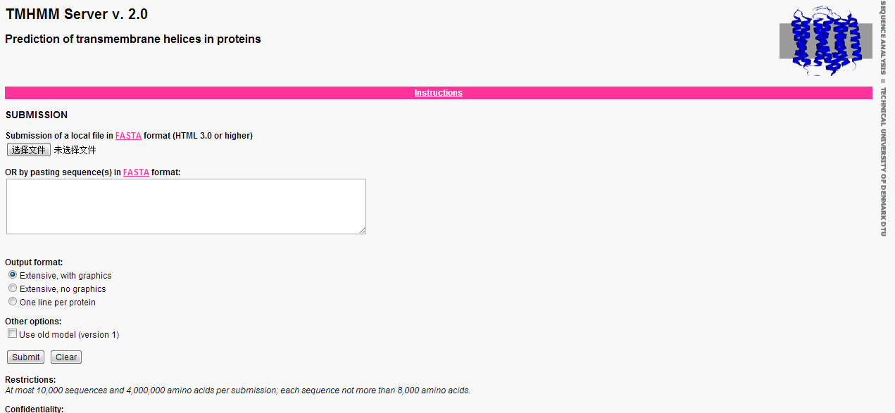
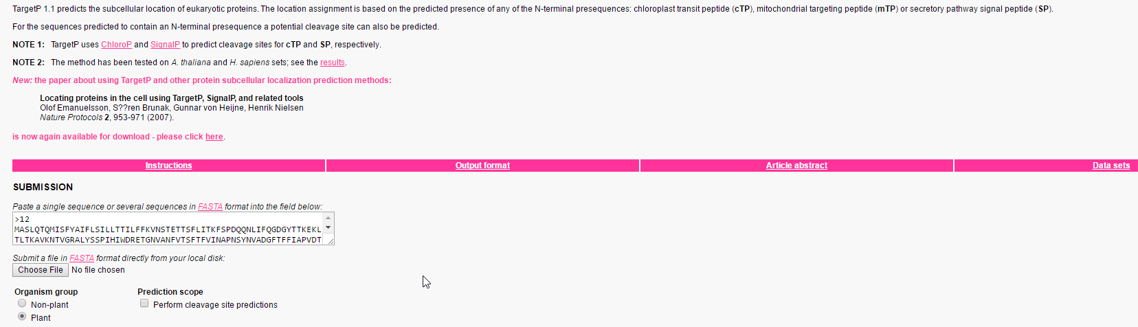
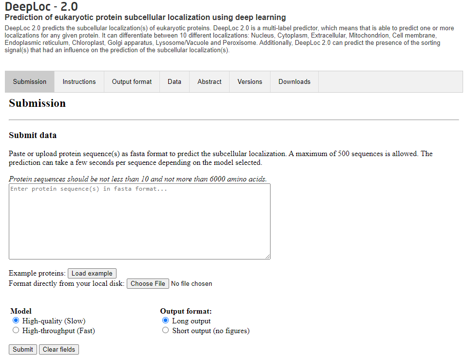
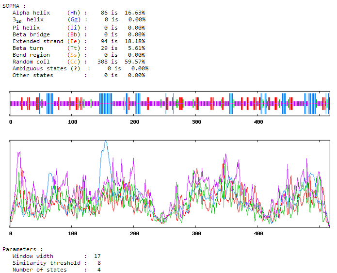

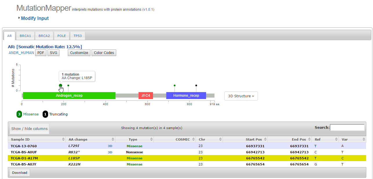

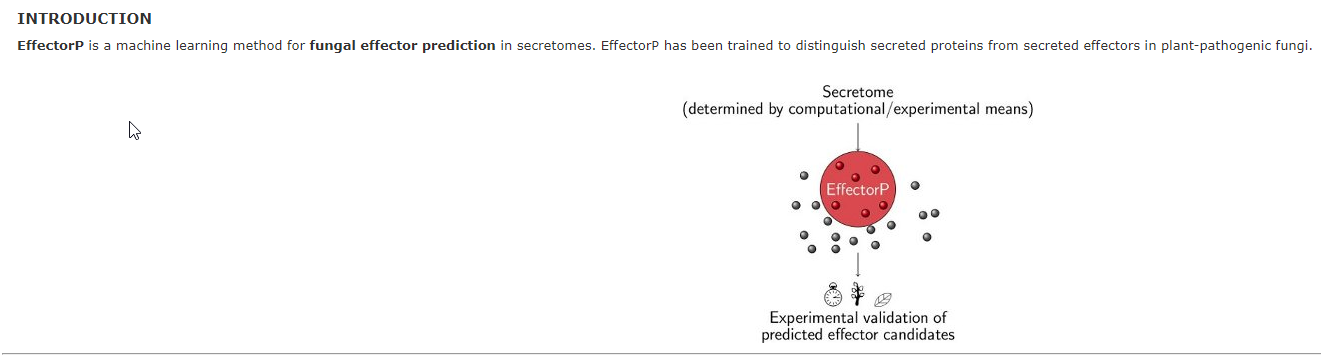

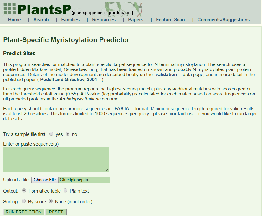
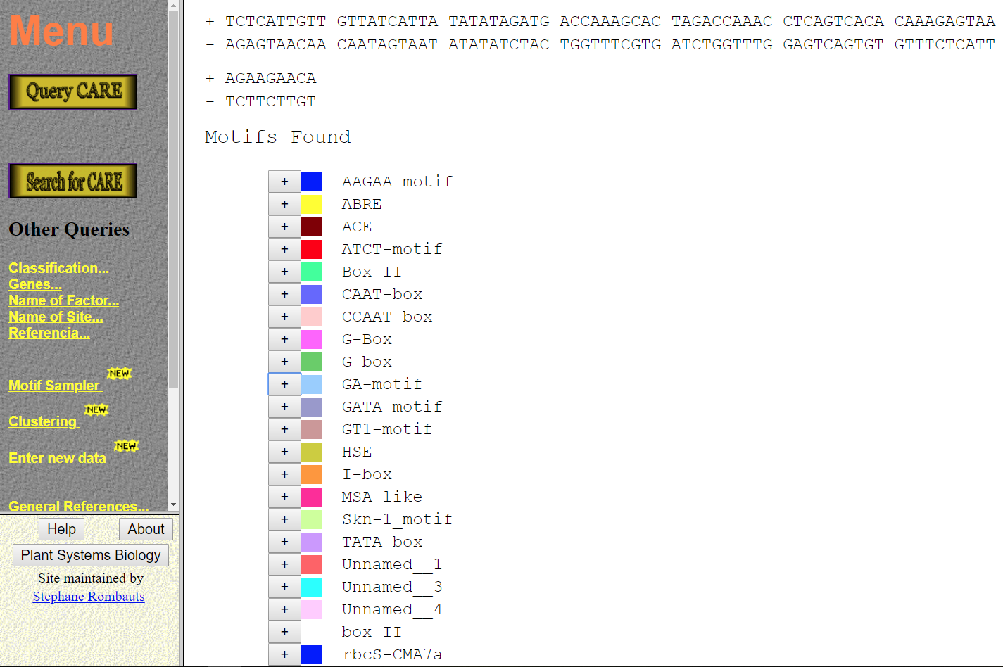
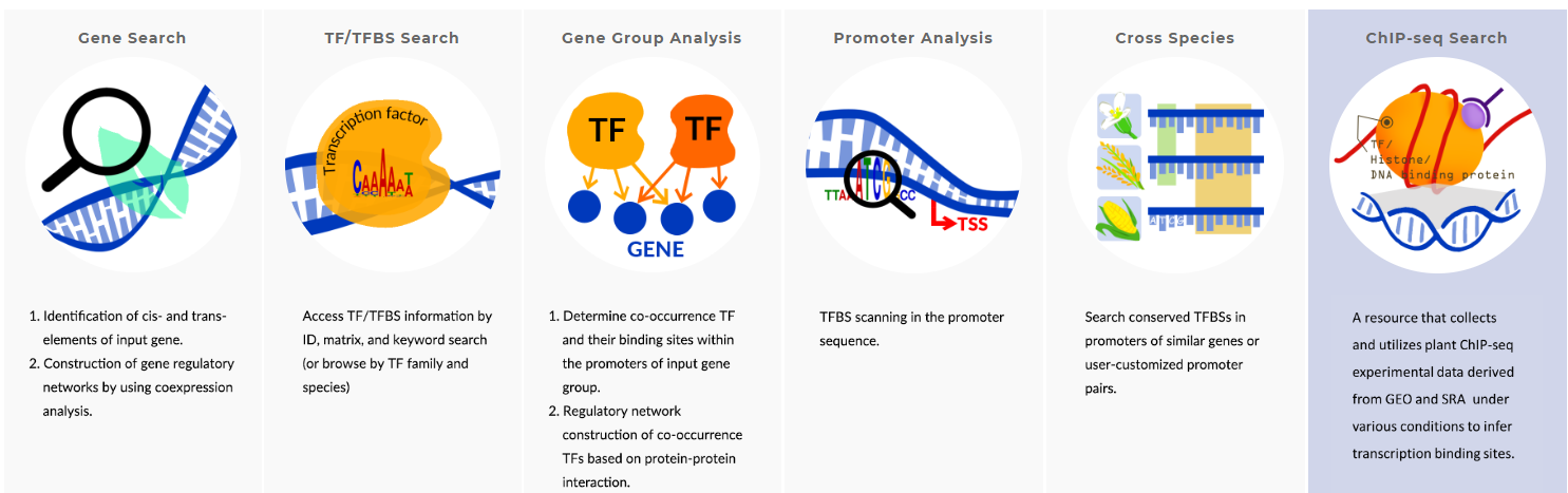
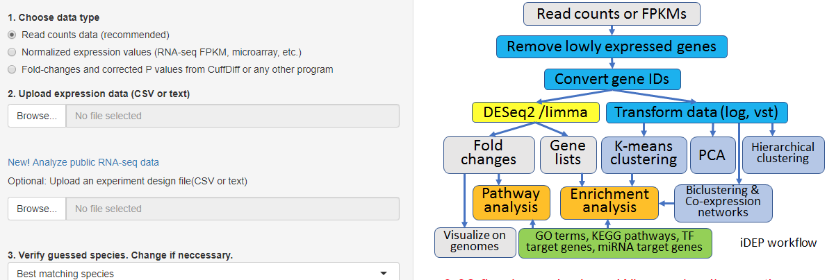
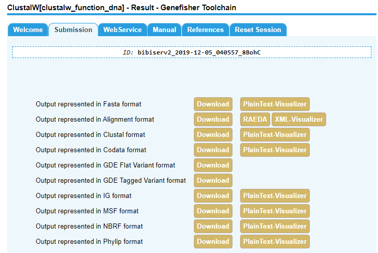


 ]]>
]]>