在重测序文章中经常见到用地图来描述测序样品分布,而地图涉及到主权,属敏感问题,但在R中可轻(fu)松(za)复现。
1. 不同方法比较
ggplot2
可灵活调整图形的任意组成成分,同时可在图形上添加2个或多个维度的数据;
maps
简单易操作,但原先中国的基础地图中,没有将四川和重庆区分开,现在虽然已经区分,但每个省份轮廓看起来还是与地图略有区别(国家基础地理信息中心);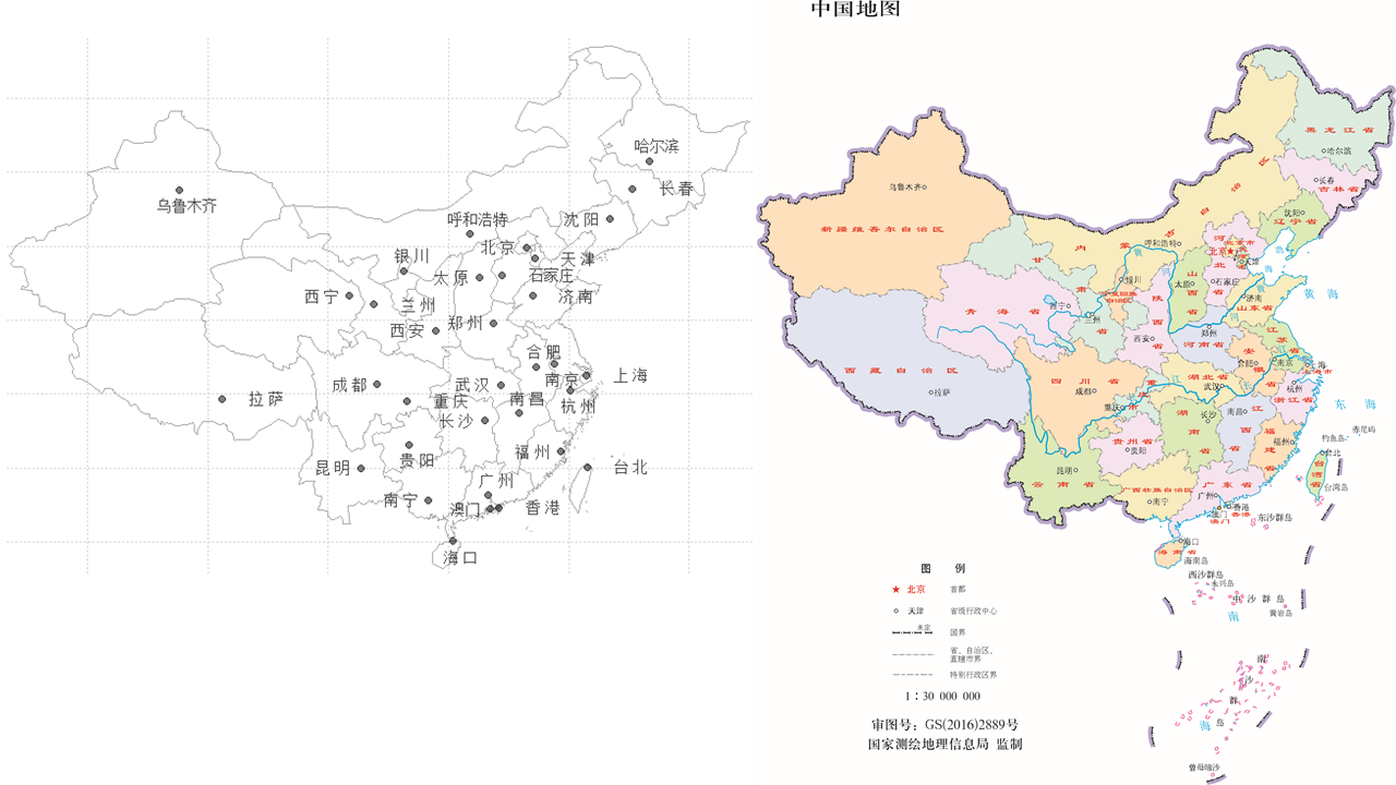
googleVis
绘制基础地图方法,仍然只能绘制一维的数据。同时绘制的地图依赖google地图;
REmap
国人开发的基于百度地图Echart。优点,绘制地图方便快捷,省市级地区的二级地图非常精准,并可绘制炫酷的迁徙图和热图,推荐学习网址:http://lchiffon.github.io/REmap/ ;缺点,同googleVis一样,只能绘制一维的数据,同时地图上只能显示中文地名。
2. 地图数据下载
Download GADM data
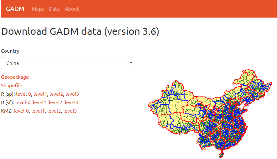
但是从GDM网站下载的中国地图没有台湾,果断差评。
GIS数据
http://cos.name/wp-content/uploads/2009/07/chinaprovinceborderdata_tar_gz.zip
主要是下载三个中国行政区地图数据信息文件: bou2_4p.dbf,bou2_4p.shp和bou2_4p.shx;
使用中如果出现中文省份名称乱码,设置Sys.setlocale("LC_ALL", "chinese")即可。
中国行政区地图数据信息数据中包含了925条记录,每条记录中都含有
面积(AREA)
周长(PERIMETER)
各种编号,ADCODE99 是国家基础地理信息中心定义的区域代码,共有 6 位数字,由省、地市、县各两位代码组成。
中文名(NAME)等字段,其中中文名(NAME)字段是以GBK编码的。可利用iconv 格式转换函数来转换各省名称table(iconv(map$NAME, from = "GBK"))
解压后三个文件放到相同目录下;虽然只读取.shp 文件,.shx 和 .dbf文件也必须在同一个文件目录下才能读取成功。
但是没有中国南海的八段线的线条绘制数据,由于南海诸岛的面积较小,如果不使用八段线标记的话,有时候如果地图展示面积太小的,南海诸岛就几乎难以辨清。
3. 地图绘制
1. Preparation
1 | setwd("F:/Rwork/china_map") |
2. Map Data
Download GIS数据:http://cos.name/wp-content/uploads/2009/07/chinaprovinceborderdata_tar_gz.zip
解压后三个文件放到当前目录(getwd())下;
虽然只读取.shp 文件,.shx 和 .dbf文件也必须在同一个文件目录下才能读取成功。1
2
3
4
5
6
7
8
9map_data <- readShapePoly("bou2_4p.shp")
names(map_data)
map_data@data$ID <- row.names(map_data@data)
map_data@data <- na.omit(map_data@data)
nrow(map_data@data)
Fmap_data <- subset(map_data, AREA > 0.005)
nrow(Fmap_data@data)
添加省会拼音
Create a data.frame called cnmapdf which contains id, prov_en and prov_cn and key map plotting info;1
2
3
4
5
6
7
8
9
10
11
12
13
14
15
16
17prov_cn <- unique(map_data$NAME)
prov_en <- c("Heilongjiang", "Inner Mongolia", "Xinjiang", "Jilin",
"Liaoning", "Gansu", "Hebei", "Beijing", "Shanxi",
"Tianjin", "Shaanxi", "Ningxia", "Qinghai", "Shandong",
"Tibet", "Henan", "Jiangsu", "Anhui", "Sichuan", "Hubei",
"Chongqing", "Shanghai", "Zhejiang", "Hunan", "Jiangxi",
"Yunnan", "Guizhou", "Fujian", "Guangxi", "Taiwan",
"Guangdong", "Hong Kong", "Hainan")
prov <- data.frame(prov_cn, prov_en)
id_prov <- map_data@data %>%
mutate(prov_en = sapply(NAME, function(x) prov$prov_en[which(prov_cn == x)])) %>%
mutate(prov_cn = as.character(NAME),prov_en = as.character(prov_en)) %>%
select(id = ID, prov_cn, prov_en)
cnmapdf <- plyr::join(fortify(map_data), id_prov, by = "id")
head(cnmapdf)
添加省会城市坐标
1 | cap_coord <- c( |
筛选南海区域和添加九段线
1 | Ncnmapdf <- cnmapdf |
3. 开始绘制地图
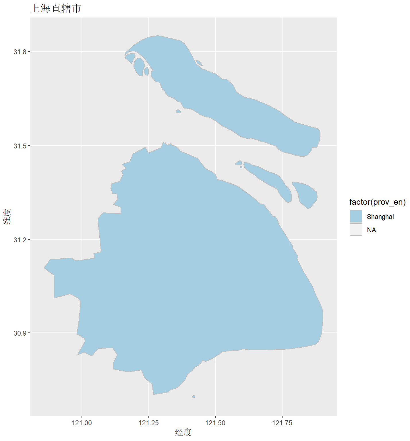
选择一个省画图
默认绘制的地图的形状有些扁平。这是因为,在绘图的过程中,默认把经度和纬度作为普通数据,均匀平等对待,绘制在笛卡尔坐标系上造成的。其实,地球的球面图形如何映射到平面图上,在地理学上是有一系列不同的专业算法的。地图不应该画在普通的笛卡尔坐标系上,而是要画在地理学专业的坐标系上。在这一点上,R 的 ggplot2 包提供了专门的coord_map()函数。1
2
3
4
5
6
7
8
9shanghai <- cnmapdf[cnmapdf$prov_en == "Shanghai",]
shanghai %>%
ggplot(aes(x = long, y = lat, group = group, fill=factor(prov_en))) +
geom_polygon( color = "grey") +
coord_map() +
ggtitle("上海直辖市") +
xlab("经度") +
ylab("维度") +
scale_fill_brewer(palette="Paired")
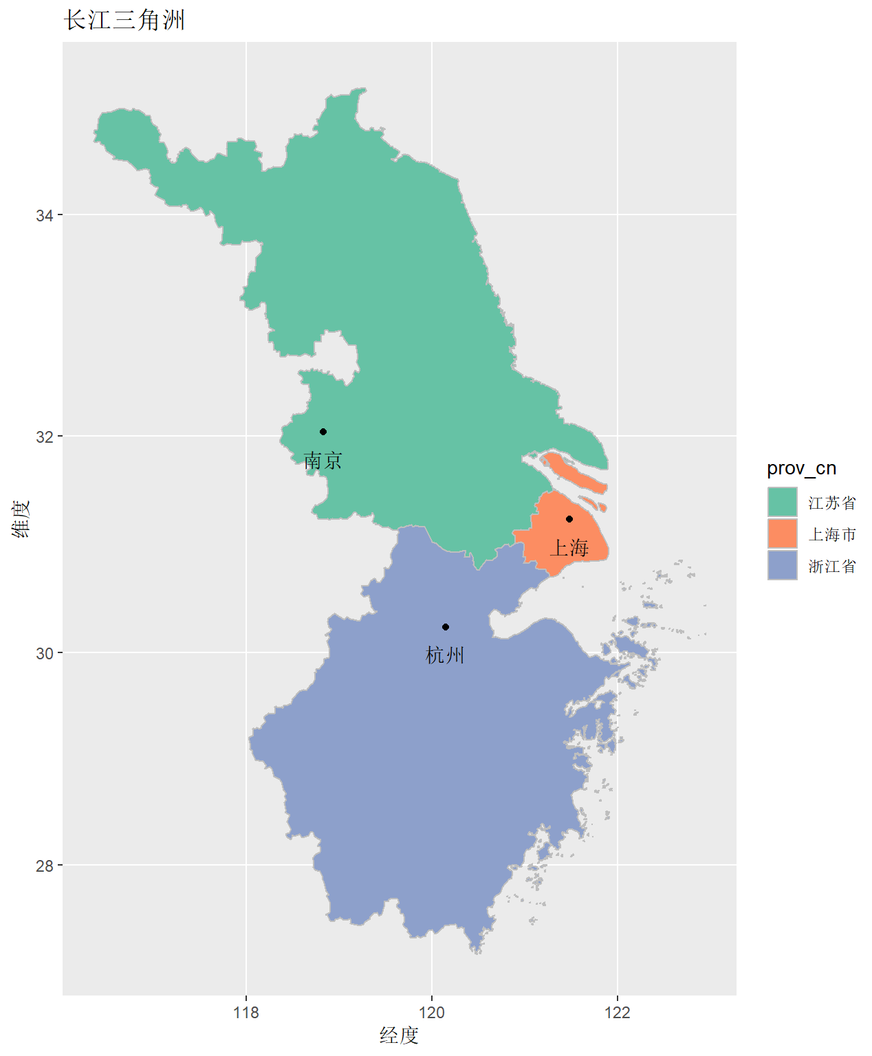
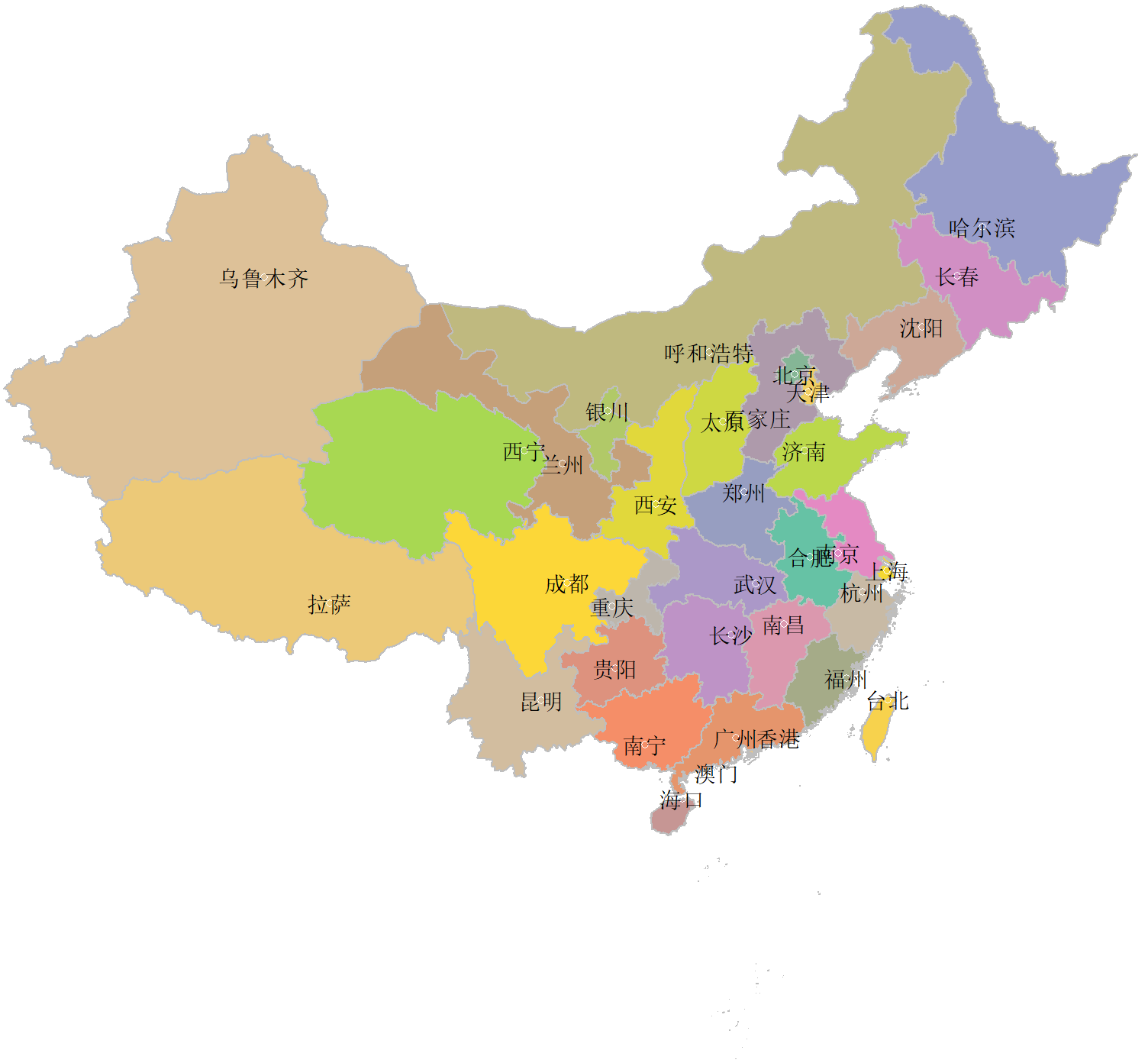
画多个省
1 | map1 <- cnmapdf %>% |
南海诸岛局部放大的全国地图
1 | nb.cols <- length(unique(Ncnmapdf$prov_en)) |
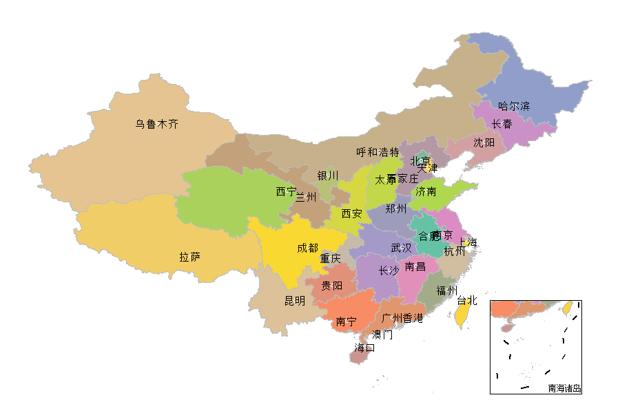
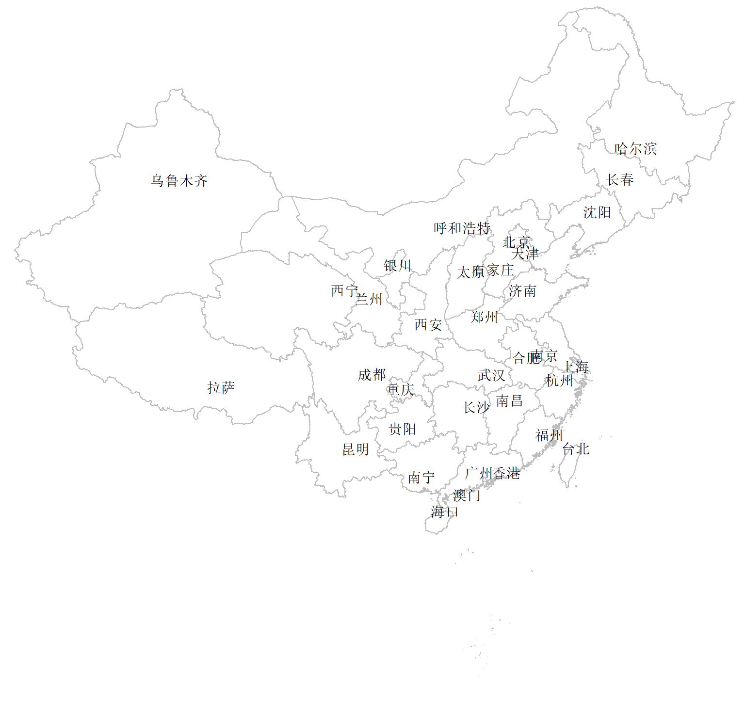
全国地图
1 | map0 <- cnmapdf %>% |
1
2
3
4
5
6
7
8
9
10
11
12
13
14
15
16
17
18
19
20map1 <- cnmapdf %>%
filter(prov_en %in% unique(cnmapdf$prov_en)) %>%
ggplot() +
geom_polygon(aes(x = long, y = lat, group = group, fill = prov_cn), color = "grey")
coord_delta_cap <- subset(cap_coord, prov_en %in% unique(cnmapdf$prov_en))
nb.cols <- length(unique(coord_delta_cap$prov_en))
mycolors <- colorRampPalette(brewer.pal(8, "Set2"))(nb.cols)
map1 +
geom_point(data = coord_delta_cap, aes(x = cap_long, y = cap_lat)) +
geom_text(data = coord_delta_cap, aes(cap_long, cap_lat - .25, label = city_cn)) +
coord_map() +
ggtitle("中国") +
xlab("经度") +
ylab("维度") +
theme_void() +
theme(legend.position = "none") +
scale_fill_manual(values = mycolors)
解决重叠地名
1 | library(ggrepel) |
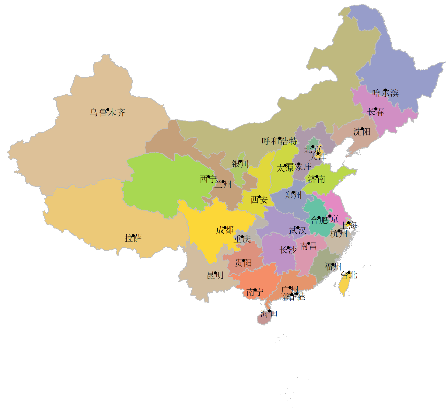
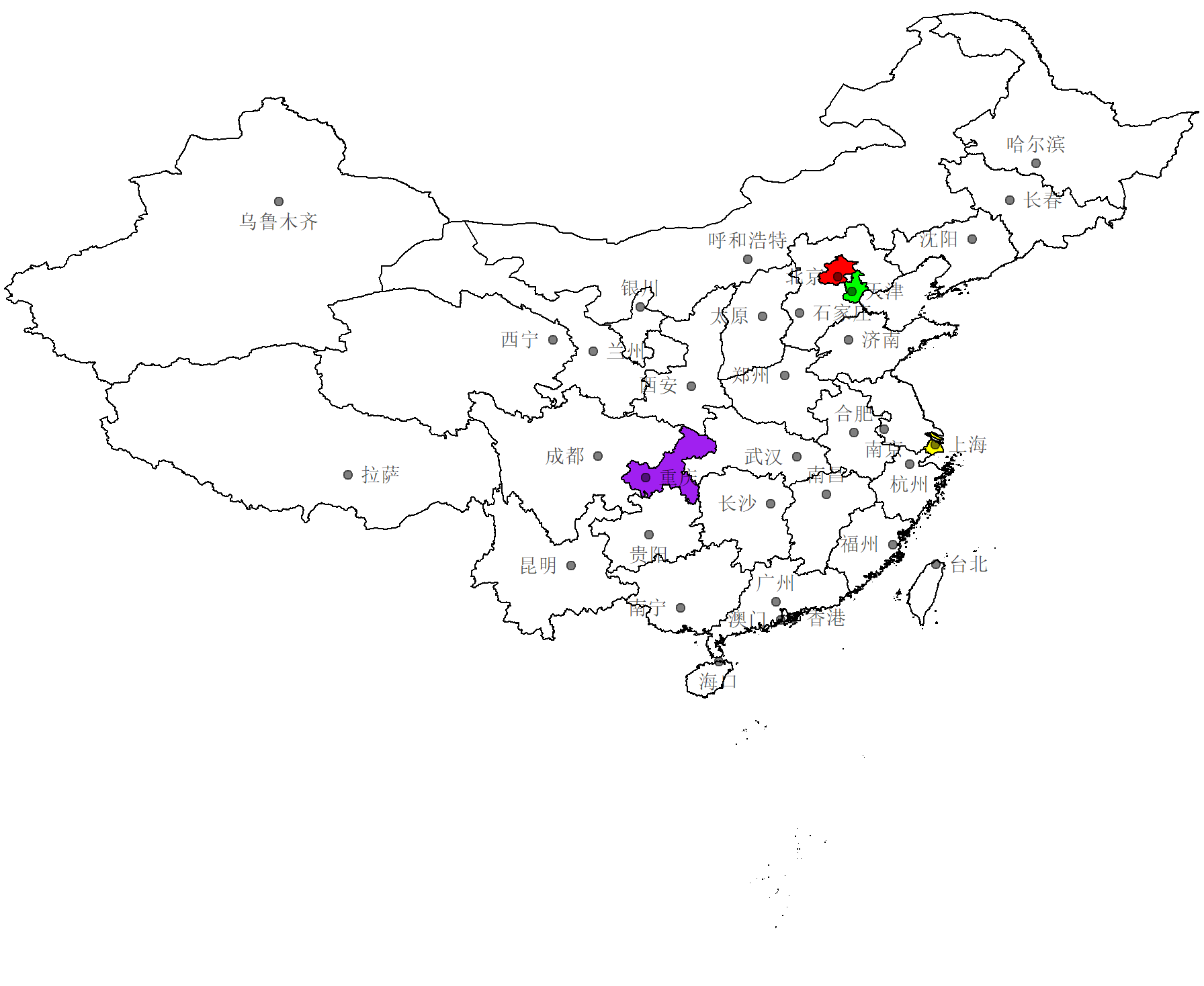
颜色标注全国地图某几个省
https://cosx.org/2009/07/drawing-china-map-using-r/1
2
3
4
5
6
7
8
9
10
11
12
13
14
15
16
17par(mar=rep(0,4))
library(maps)
library(mapdata)
getColor = function(mapdata, provname, provcol, othercol){
f = function(x, y) ifelse(x %in% y, which(y == x), 0)
colIndex = sapply(mapdata@data$NAME, f, provname)
fg = c(othercol, provcol)[colIndex + 1]
return(fg)
}
provname = c("北京市", "天津市", "上海市", "重庆市")
provcol = c("red", "green", "yellow", "purple")
plot(map_data, col = getColor(map_data, provname, provcol, "white"))
points(cap_coord$cap_long, cap_coord$cap_lat, pch = 19, col = rgb(0, 0, 0, 0.5))
text(cap_coord$cap_long, cap_coord$cap_lat, cap_coord[, 3], cex = 0.9, col = rgb(0,0, 0, 0.7),
pos = c(2, 4, 4, 4, 3, 4, 2, 3, 4, 2, 4, 2, 2, 4, 3, 2, 1, 3, 1, 1, 2, 3, 2, 2, 1, 2, 4, 3, 1, 2, 2, 4, 4, 2))
axis(1, lwd = 0); axis(2, lwd = 0); axis(3, lwd = 0); axis(4, lwd = 0)
as.character(na.omit(unique(map_data@data$NAME)))
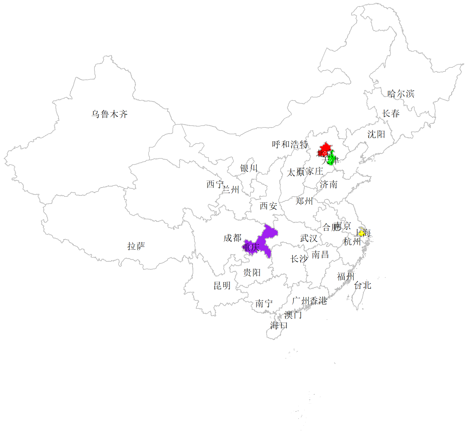
颜色标注全国地图某几个省 (推荐)
1 | provname = c("北京市", "天津市", "上海市", "重庆市") |
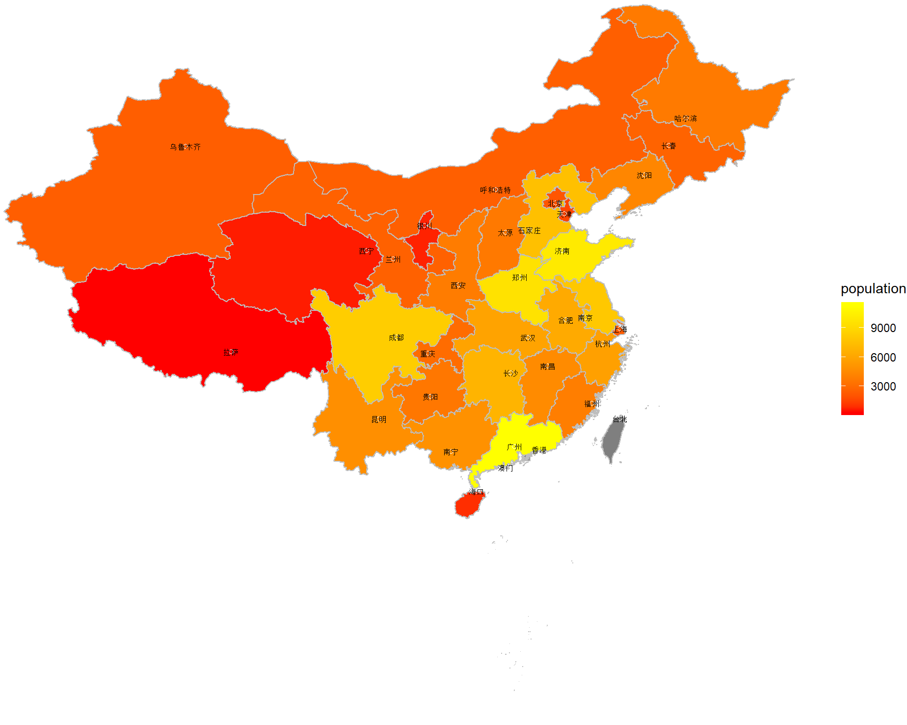
4. 地图添加数据
实例数据下载:中华人民共和国国家统计局
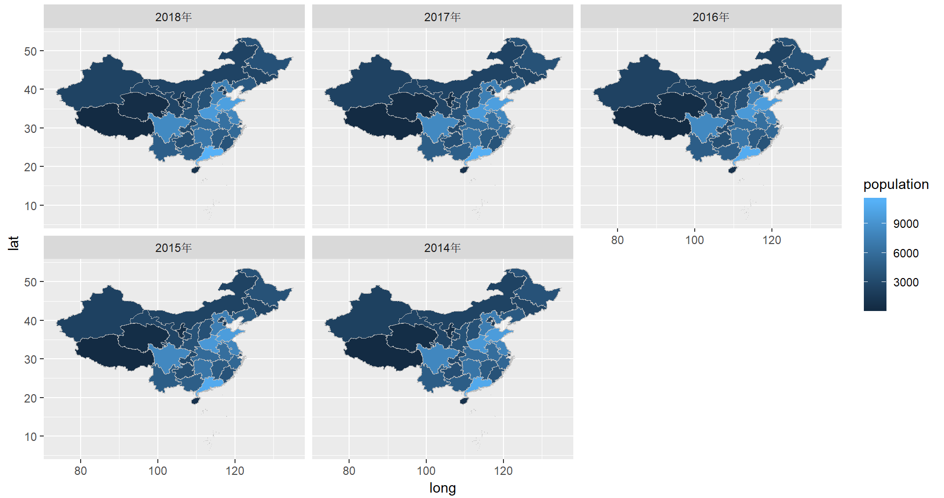
Heatmap
1 | democn <- read.csv("China_pop.csv", stringsAsFactors = F, check.names=FALSE) |
多个图1
2
3
4
5
6
7
8
9map3df <- cnmapdf %>%
plyr::join(democndf, by = "prov_cn") %>%
mutate(population = as.numeric(population)) %>%
na.omit()
map3df %>%
ggplot(aes(x = long, y = lat, group = group, fill = population)) +
geom_polygon(color = "grey", lwd = .1) +
coord_equal() +
facet_wrap(~year)
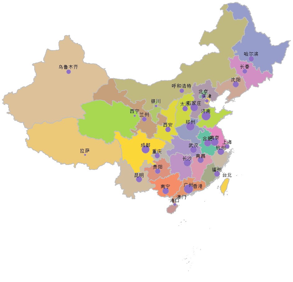
Bubbles
1 | map1 + |
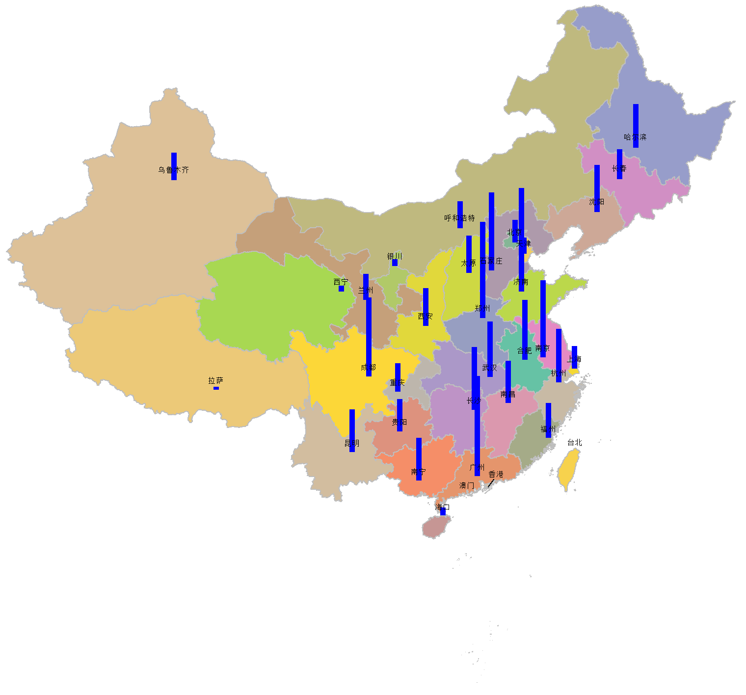
Bar
1 | map1 + |
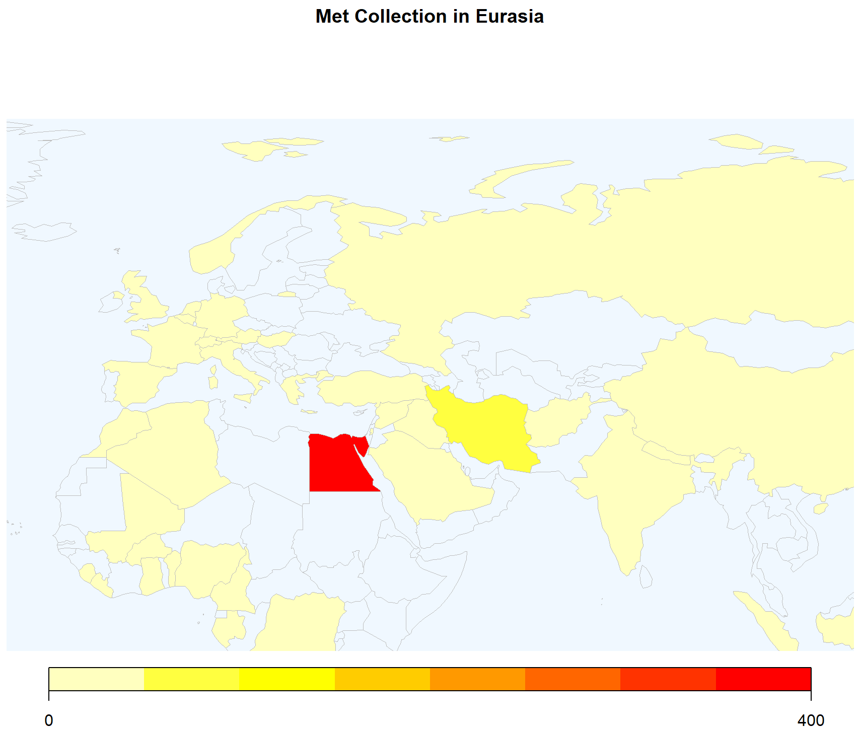
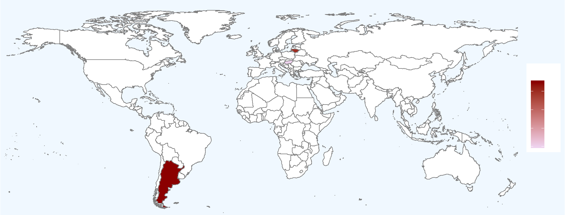
5. 世界地图
1 | library(rworldmap) |
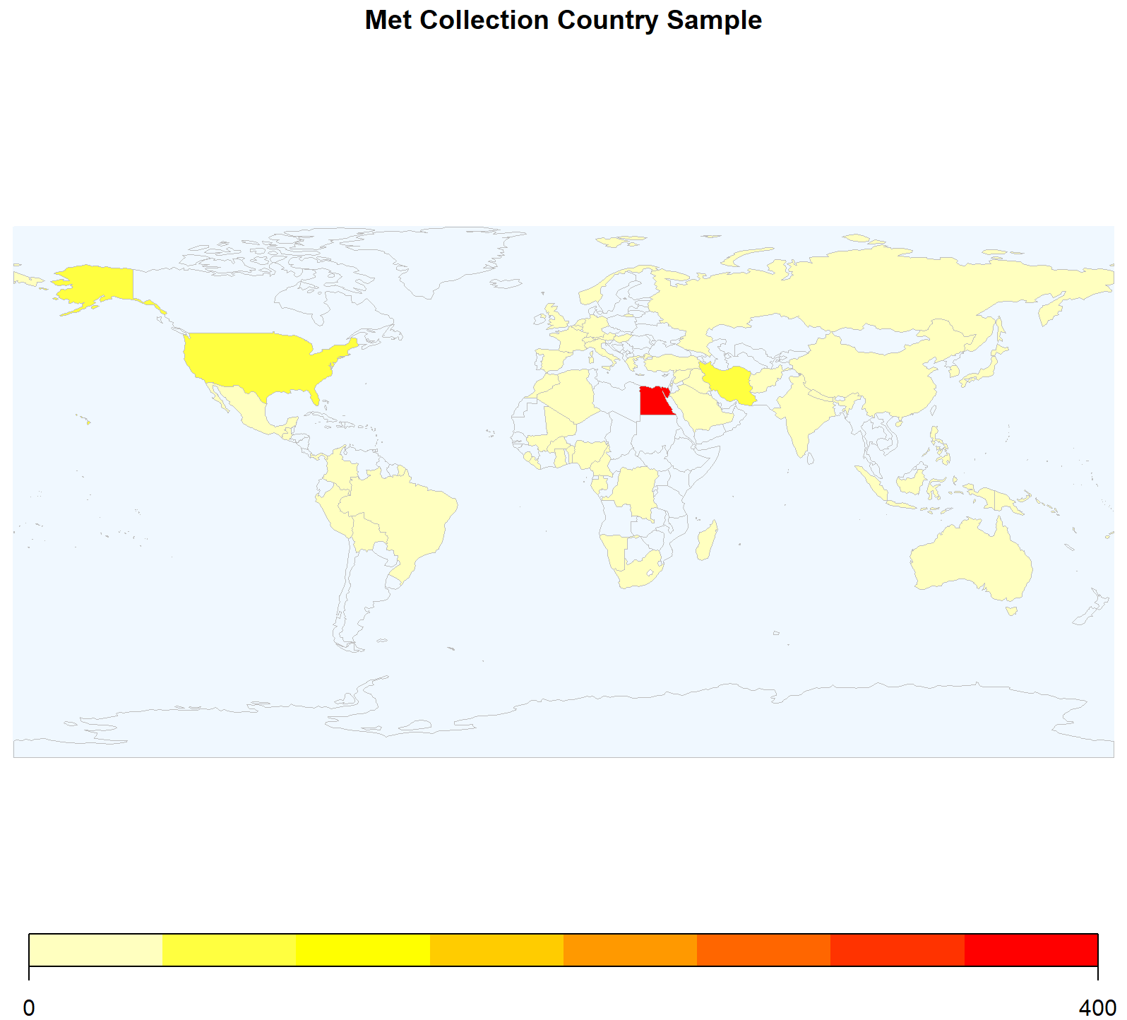
仅显示某一区域
1 | mapCountryData(matched, nameColumnToPlot="value", mapTitle="Met Collection in Eurasia", mapRegion="Eurasia", colourPalette="heat", catMethod="pretty", oceanCol="aliceblue") |
1
2
3
4
5
6
7
8
9
10
11
12
13
14
15
16
17
18
19
20
21
22
23
24
25
26
27
28
29
30
31
32library(ggplot2)
library(dplyr)
WorldData <- map_data('world') %>% filter(region != "Antarctica") %>% fortify
df <- data.frame(region=c('Hungary','Lithuania','Argentina'),
value=c(4,10,11),
stringsAsFactors=FALSE)
p <- ggplot() +
geom_map(data = WorldData, map = WorldData,
aes(x =long , y = lat, group = group, map_id=region),
fill = "white", colour = "#7f7f7f", size=0.5) +
geom_map(data = df, map=WorldData, aes(fill=value, map_id=region),colour="#7f7f7f", size=0.5) +
coord_map("rectangular", lat0=0, xlim=c(-180,180), ylim=c(-60, 90)) +
scale_fill_continuous(low="thistle2", high="darkred", guide="colorbar") +
scale_y_continuous(breaks=c()) +
scale_x_continuous(breaks=c()) +
labs(fill="legend", title="Title", x="", y="") +
theme(text = element_text( color = "#FFFFFF")
,panel.background = element_rect(fill = "aliceblue")
,plot.background = element_rect(fill = "aliceblue")
,panel.grid = element_blank()
,plot.title = element_text(size = 30)
,plot.subtitle = element_text(size = 10)
,axis.text = element_blank()
,axis.title = element_blank()
,axis.ticks = element_blank()
,legend.position = "right"
)
#theme_bw()
p
6. Info
1 | # R version 3.4.2 (2017-09-28) |
4. 参考
R Visual. - China Map Part II
https://www.datanovia.com/en/blog/ggplot-colors-best-tricks-you-will-love/
https://www.datanovia.com/en/blog/top-r-color-palettes-to-know-for-great-data-visualization/
标准中国地图的绘制