1 | > text1<-read.delim("fun.txt",header=FALSE) |
关键点解释
设置图形参数—函数par()1
2
3
4
5
6
7adj:设定在text、mtext、title中字符串的对齐方向。0表示左对齐,0.5(默认值)表示居中,而1表示右对齐。
ann:如果ann=FALSE,那么高水平绘图函数会调用函数plot.default使对坐标轴名称、整体图像名称不做任何注解。
bty:用于限定图形的边框类型。如果bty的值为"o"(默认值)、"l"、"7"、"c"、"u"或者"]"中的任意一个,对应的边框类型就和该字母的形状相似,"n",表示无边框。
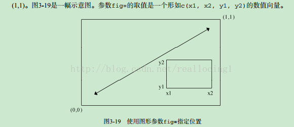
fig: c(x1, x2, y1, y2),设定当前图形在绘图设备中所占区域,需要满足x1<x2,y1<y2。如果修改参数fig,会自动打开一个新的绘图设备,而若希望在原来的绘图设备中添加新的图形,需要和参数new=TRUE一起使用。
fin:当前绘图区域的尺寸规格,形式为(width,height)。
lty:直线类型。参数的值可以为整数(0为空,1为实线(默认值),2为虚线,3为点线。
oma:参数形式为c(bottom, left, top, right) ,用于设定外边界。
melt()1
2id.vars 是被当做维度的列变量,每个变量在结果中占一列;
measure.vars 是被当成观测值的列变量,它们的列变量名称和值分别组成 variable 和 value两列,列变量名称用variable.name 和 value.name来指定。
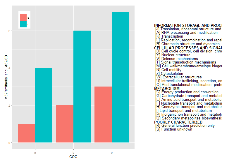
position()1
2
3
4
5
6geom_bar(position="dodge")调整条形图排列方式,可选参数为"dodge,fill,identity,jitter,stack"。legend.position调整图例位置。
dodge:"避让"方式,即往旁边闪,如柱形图的并排方式就是这种
fill:填充方式, 先把数据归一化,再填充到绘图区的顶部
identity:原地不动,不调整位置
jitter:随机抖一抖,让本来重叠的露出点头来
stack:叠罗汉
1 | b<-20;为自定义值,根据图形微调。 |
1 | 1,7,18,27为文本文件中特殊行。 |
附加
通过设置par()绘制一页多图1
2
3
4
5
6
7
8
9
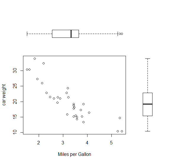
10attach(mtcars)
opar<-par(no.readonly=T)
par(fig=c(0,0.8,0,0.8))
plot(wt,mpg,xlab="Miles per Gallon",ylab="car weight")
par(fig=c(0,0.8,0.55,1),new=T)
boxplot(wt,horizontal=T,axes=F)
par(fig=c(0.65,1,0,0.8),new=T)
boxplot(mpg,axes=F)
par(opar)
detach(mtcars)
Contribution from :http://www.dataguru.cn/article-4827-1.html