Description
Methods for Cluster analysis. Much extended the original from Peter Rousseeuw, Anja Struyf and Mia Hubert, based on Kaufman and Rousseeuw (1990) ``Finding Groups in Data’’.
聚类分析:按照个体或样品(individuals, objects or subjects)的特征将它们分类,使同一类别内的个体具有尽可能高的同质性(homogeneity),而类别之间则应具有尽可能高的异质性(heterogeneity)。
Cluster analysis or clustering is the task of grouping a set of objects in such a way that objects in the same group (called a cluster) are more similar (in some sense or another) to each other than to those in other groups (clusters). It is a main task of exploratory data mining, and a common technique for statistical data analysis, used in many fields, including machine learning, pattern recognition, image analysis, information retrieval, and bioinformatics.
Typical cluster models
Algorithms
Connectivity based clustering (hierarchical clustering)
Connectivity based clustering, also known as hierarchical clustering, is based on the core idea of objects being more related to nearby objects than to objects farther away. These algorithms connect “objects” to form “clusters” based on their distance. A cluster can be described largely by the maximum distance needed to connect parts of the cluster. At different distances, different clusters will form, which can be represented using a dendrogram, which explains where the common name “hierarchical clustering” comes from: these algorithms do not provide a single partitioning of the data set, but instead provide an extensive hierarchy of clusters that merge with each other at certain distances. In a dendrogram, the y-axis marks the distance at which the clusters merge, while the objects are placed along the x-axis such that the clusters don’t mix.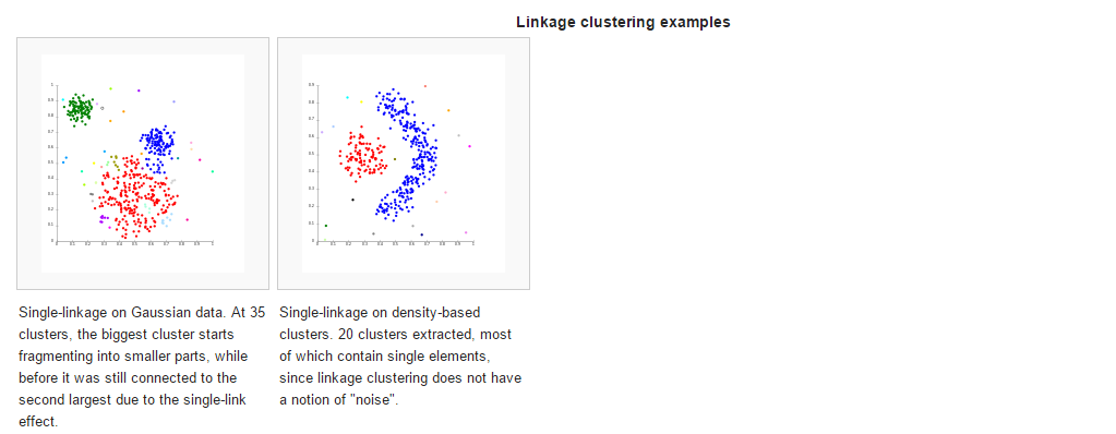
Centroid-based clustering
In centroid-based clustering, clusters are represented by a central vector, which may not necessarily be a member of the data set. When the number of clusters is fixed to k, k-means clustering gives a formal definition as an optimization problem: find the k cluster centers and assign the objects to the nearest cluster center, such that the squared distances from the cluster are minimized.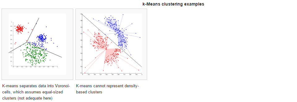
Distribution-based clustering
The clustering model most closely related to statistics is based on distribution models. Clusters can then easily be defined as objects belonging most likely to the same distribution. A convenient property of this approach is that this closely resembles the way artificial data sets are generated: by sampling random objects from a distribution.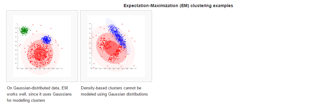
Density-based clustering
The most popular density based clustering method is DBSCAN. In contrast to many newer methods, it features a well-defined cluster model called “density-reachability”. Similar to linkage based clustering, it is based on connecting points within certain distance thresholds. However, it only connects points that satisfy a density criterion, in the original variant defined as a minimum number of other objects within this radius.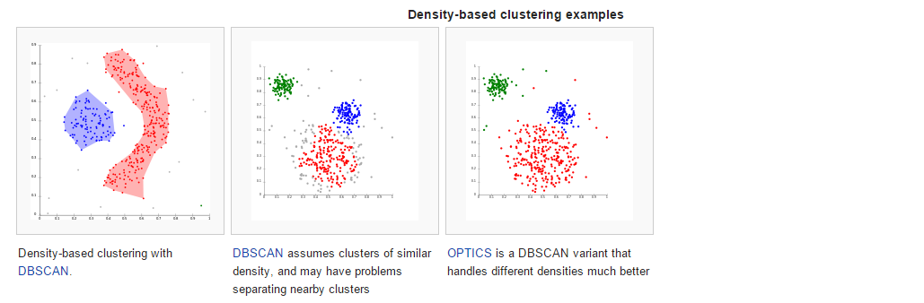
综上内容看出其和主成份分析(Principal component analysis,PCA)有较多相似性,所以开始前先对主成份分析、因子分析和聚类分析的异同点进行比较分析,具体关于PCA分析可看本博博文PCA分析。
R中进行聚类分析
cluster包
1 | > library(cluster) |
参数解释:
daisy:Dissimilarity Matrix(相异度矩阵)Calculation,compute all the pairwise dissimilarities (distances) between observations in the data set.
相异度矩阵:相异度矩阵是对象—对象结构的一种数据表达方式,多数聚类算法都是建立在相异度矩阵基础上,如果数据是以数据矩阵形式给出的,就要将数据矩阵转化为相异度矩阵。对象间的相似度或相异度是基于两个对象间的距离来计算的。1
daisy(x, metric = c("euclidean", "manhattan", "gower"),stand = FALSE, type = list(), weights = rep.int(1, p))
x—numeric matrix or data frame, of dimension n*p.
metric—“euclidean” (the default), “manhattan” and “gower”.Euclidean distances are root sum-of-squares of differences, and manhattan distances
are the sum of absolute differences.”Gower’s distance” is chosen by metric “gower” or automatically if some columns of x are not numeric.
stand—logical flag: if TRUE, then the measurements in x are standardized before calculating the dissimilarities. Measurements are standardized for each variable (column), by subtracting the variable’s mean value and dividing by the variable’s mean absolute deviation.
pam:Partitioning (clustering) of the data into k clusters “around medoids”, a more robust version of K-means.1
2
3
4
5
6pam(x, k, diss = inherits(x, "dist"), metric = "euclidean",
medoids = NULL, stand = FALSE, cluster.only = FALSE,
do.swap = TRUE,
keep.diss = !diss && !cluster.only && n < 100,
keep.data = !diss && !cluster.only,
pamonce = FALSE, trace.lev = 0)
x—data matrix or data frame, or dissimilarity matrix or object.In case of a dissimilarity matrix, x is typically the output of daisy or dist.
k—positive integer specifying the number of clusters, less than the number of observations.
diss—logical flag: if TRUE (default for dist or dissimilarity objects), then x will be considered as a dissimilarity matrix. If FALSE, then x will be considered as a matrix of observations by variables.
metric—“euclidean” and “manhattan”,If x is already a dissimilarity matrix, then this argument will be ignored.
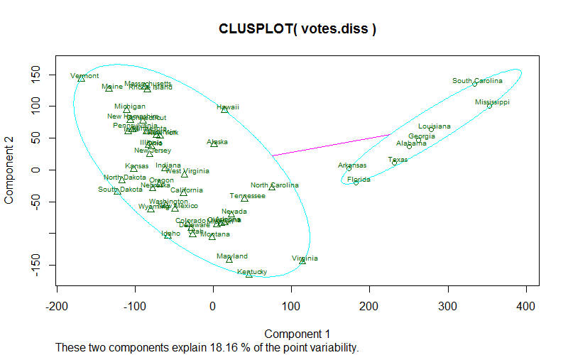
clusplot:Bivariate Cluster Plot (clusplot) Default Method1
2
3
4
5
6
7
8
9
10
11
12
13
14
15clusplot(x, clus, diss = FALSE,
s.x.2d = mkCheckX(x, diss), stand = FALSE,
lines = 2, shade = FALSE, color = FALSE,
labels= 0, plotchar = TRUE,
col.p = "dark green", col.txt = col.p,
col.clus = if(color) c(2, 4, 6, 3) else 5, cex = 1, cex.txt = cex,
span = TRUE,
add = FALSE,
xlim = NULL, ylim = NULL,
main = paste("CLUSPLOT(", deparse(substitute(x)),")"),
sub = paste("These two components explain",
round(100 * var.dec, digits = 2), "% of the point variability."),
xlab = "Component 1", ylab = "Component 2",
verbose = getOption("verbose"),
...)
x—data matrix or data frame, or dissimilarity matrix or object.In case of a dissimilarity matrix, x is typically the output of daisy or dist.
clus—clus is often the clustering component of the output of pam.
diss—logical flag: if TRUE (default for dist or dissimilarity objects), then x will be considered as a dissimilarity matrix. If FALSE, then x will be considered as a matrix of observations by variables.
lines—lines = 0, no distance lines will appear on the plot;lines = 1, the line segment between m1 and m2 is drawn;lines = 2, a line segment between the boundaries of E1 and E2 is drawn (along the line connecting m1 and m2).
shade—logical flag: if TRUE, then the ellipses are shaded in relation to their density.
color—logical flag: if TRUE, then the ellipses are colored with respect to their density.labels—labels= 0, no labels are placed in the plot;
labels= 1, points and ellipses can be identified in the plot (see identify);labels= 2, all points and ellipses are labelled in the plot;labels= 3, only the points are labelled in the plot;labels= 4, only the ellipses are labelled in the plot.labels= 5, the ellipses are labelled in the plot, and points can be identified.
col.p—color code(s) used for the observation points.
更多资源
https://cran.r-project.org/web/views/Cluster.html