hope

A new day is coming,whether we like it or not. The question is will you control it,or will it control you?


  • Home

  • Archives

  • Code

  • Categories

  • Tags

  • Footprint

  • qRT-PCR

  • Project

  • Publish

  • SCI Figure

  • About

  • CV

  • Search

ggplot2 error bars (finished)-Quick start guide - R software and data visualization

Posted on 2015-09-21 | In R | Comments: | Views: ℃
| Words count in article: | Reading time ≈

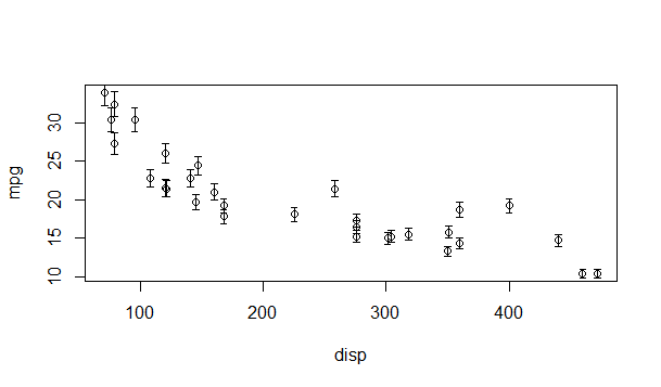
This tutorial describes how to create a graph with error bars using R software and ggplot2 package. There are different types of error bars which can be created using the functions below :


  • geom_errorbar()

  • geom_linerange()

  • geom_pointrange()

  • geom_crossbar()

  • geom_errorbarh()


Add error bars to a bar and line plots


Prepare the data


ToothGrowth data is used. It describes the effect of Vitamin C on tooth growth in Guinea pigs. Three dose levels of Vitamin C (0.5, 1, and 2 mg) with each of two delivery methods [orange juice (OJ) or ascorbic acid (VC)] are used :


1
2
3
4
5
6
7
8
9
10
11
library(ggplot2)
df <- ToothGrowth
df$dose <- as.factor(df$dose)
head(df)
len supp dose
1 4.2 VC 0.5
2 11.5 VC 0.5
3 7.3 VC 0.5
4 5.8 VC 0.5
5 6.4 VC 0.5
6 10.0 VC 0.5


  • len : Tooth length

  • dose : Dose in milligrams (0.5, 1, 2)

  • supp : Supplement type (VC or OJ)

  • In the example below, we’ll plot the mean value of Tooth length in each group. The standard deviation is used to draw the error bars on the graph.


    First, the helper function below will be used to calculate the mean and the standard deviation, for the variable of interest, in each group :


    1
    2
    3
    4
    5
    6
    7
    8
    9
    10
    11
    12
    13
    14
    15
    16
    17
    18
    19
    20
    #+++++++++++++++++++++++++
    # Function to calculate the mean and the standard deviation
    # for each group
    #+++++++++++++++++++++++++
    # data : a data frame
    # varname : the name of a column containing the variable
    #to be summariezed
    # groupnames : vector of column names to be used as
    # grouping variables
    data_summary <- function(data, varname, groupnames){
    require(plyr)
    summary_func <- function(x, col){
    c(mean = mean(x[[col]], na.rm=TRUE),
    sd = sd(x[[col]], na.rm=TRUE))
    }
    data_sum<-ddply(data, groupnames, .fun=summary_func,
    varname)
    data_sum <- rename(data_sum, c("mean" = varname))
    return(data_sum)
    }


    Summarize the data :


    1
    2
    3
    4
    5
    6
    7
    8
    9
    10
    11
    12
    df2 <- data_summary(ToothGrowth, varname="len", 
    groupnames=c("supp", "dose"))
    # Convert dose to a factor variable
    df2$dose=as.factor(df2$dose)
    head(df2)
    supp dose len sd
    1 OJ 0.5 13.23 4.459709
    2 OJ 1 22.70 3.910953
    3 OJ 2 26.06 2.655058
    4 VC 0.5 7.98 2.746634
    5 VC 1 16.77 2.515309
    6 VC 2 26.14 4.797731


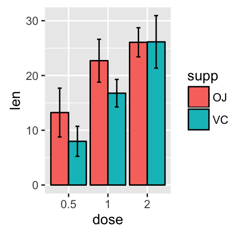
    Barplot with error bars


    The function geom_errorbar() can be used to produce the error bars :


    1
    2
    3
    4
    5
    6
    7
    8
    9
    10
    11
    12
    13
    library(ggplot2)
    # Default bar plot
    p<- ggplot(df2, aes(x=dose, y=len, fill=supp)) +
    geom_bar(stat="identity", color="black",
    position=position_dodge()) +
    geom_errorbar(aes(ymin=len-sd, ymax=len+sd), width=.2,
    position=position_dodge(.9))
    print(p)

    # Finished bar plot
    p+labs(title="Tooth length per dose", x="Dose (mg)", y = "Length")+
    theme_classic() +
    scale_fill_manual(values=c('#999999','#E69F00'))


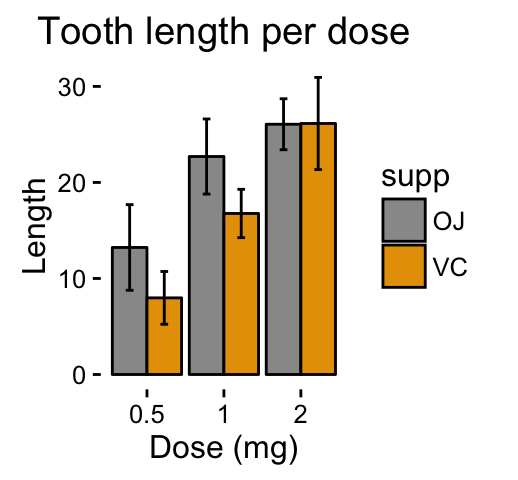
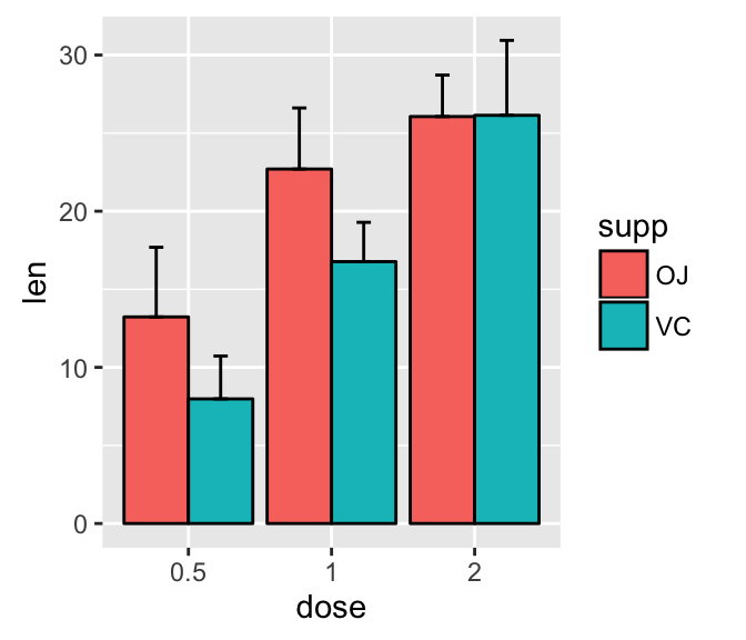
    Note that, you can chose to keep only the upper error bars
    1
    2
    3
    4
    5
    # Keep only upper error bars
    ggplot(df2, aes(x=dose, y=len, fill=supp)) +
    geom_bar(stat="identity", color="black", position=position_dodge()) +
    geom_errorbar(aes(ymin=len, ymax=len+sd), width=.2,
    position=position_dodge(.9))


    Read more on ggplot2 bar graphs : ggplot2 bar graphs


    Line plot with error bars


    1
    2
    3
    4
    5
    6
    7
    8
    9
    10
    11
    12
    # Default line plot
    p<- ggplot(df2, aes(x=dose, y=len, group=supp, color=supp)) +
    geom_line() +
    geom_point()+
    geom_errorbar(aes(ymin=len-sd, ymax=len+sd), width=.2,
    position=position_dodge(0.05))
    print(p)

    # Finished line plot
    p+labs(title="Tooth length per dose", x="Dose (mg)", y = "Length")+
    theme_classic() +
    scale_color_manual(values=c('#999999','#E69F00'))


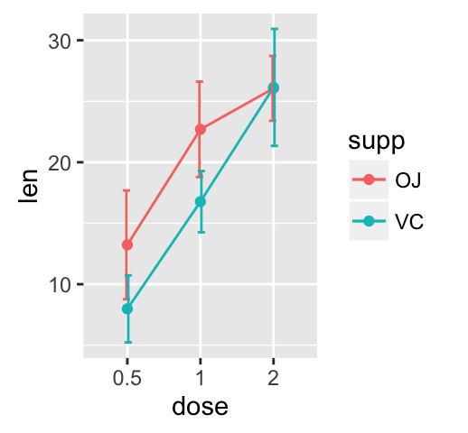
    You can also use the functions geom_pointrange() or geom_linerange() instead of using geom_errorbar()


    1
    2
    3
    4
    5
    6
    7
    8
    # Use geom_pointrange
    ggplot(df2, aes(x=dose, y=len, group=supp, color=supp)) +
    geom_pointrange(aes(ymin=len-sd, ymax=len+sd))

    # Use geom_line()+geom_pointrange()
    ggplot(df2, aes(x=dose, y=len, group=supp, color=supp)) +
    geom_line()+
    geom_pointrange(aes(ymin=len-sd, ymax=len+sd))


    Read more on ggplot2 line plots : ggplot2 line plots


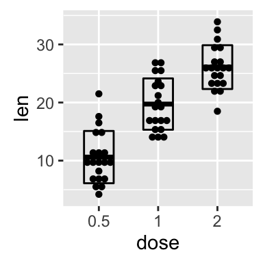
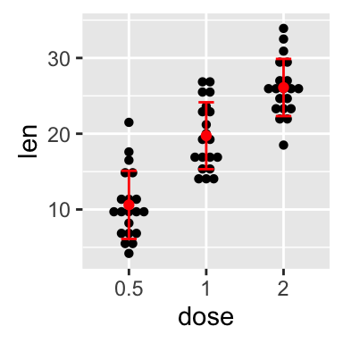
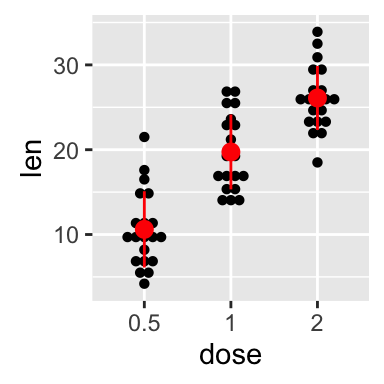
    Dot plot with mean point and error bars


    The functions geom_dotplot() and stat_summary() are used :


    The mean +/- SD can be added as a crossbar , a error bar or a pointrange :


    1
    2
    3
    4
    5
    6
    7
    8
    9
    10
    11
    12
    13
    14
    15
    p <- ggplot(df, aes(x=dose, y=len)) + 
    geom_dotplot(binaxis='y', stackdir='center')

    # use geom_crossbar()
    p + stat_summary(fun.data="mean_sdl", mult=1,
    geom="crossbar", width=0.5)

    # Use geom_errorbar()
    p + stat_summary(fun.data=mean_sdl, mult=1,
    geom="errorbar", color="red", width=0.2) +
    stat_summary(fun.y=mean, geom="point", color="red")

    # Use geom_pointrange()
    p + stat_summary(fun.data=mean_sdl, mult=1,
    geom="pointrange", color="red")


    Read more on ggplot2 dot plots : ggplot2 dot plot


    Infos


    This analysis has been performed using R software (ver. 3.1.2) and ggplot2 (ver. 1.0.0)

    Contribution from :http://www.sthda.com/english/wiki/ggplot2-error-bars-quick-start-guide-r-software-and-data-visualization

    CRISPR/Cas9

    Posted on 2015-09-13 | In Bioinformatics | Comments: | Views: ℃
    | Words count in article: | Reading time ≈

    CRISPR/Cas9 gene editing technology has revolutionized the field of genome modification. This system is based on two key components that form a complex: Cas9 endonuclease and a target-specific RNA (single guide RNA or sgRNA) that guides Cas9 to the genomic DNA target site. Targeting to a particular genomic locus is solely mediated by the sgRNA.

    CRISPR/Cas9 简介

    细菌(bacteria)和古细菌(archaea)都有一套防御机制抵御这种外来的侵入性因子,这种防御机制就是在成簇的、有规律间隔的多次重复短片段(clustered regularly interspaced short palindromic repeat, CRISPR)的基础上建立起来的适应性免疫系统(adaptive immune system)。
    CRISPR系统能够将各种外源的病毒或质粒DNA短片段”集中”到细胞基因组里某个特定的重复片段区域上,将这些外源DNA当作细胞曾经经受过外源DNA入侵的一种记忆给储存起来。然后这段DNA会转录生成CRISPR前体RNA(precursor CRISPR RNA),前体RNA生成之后会被切割成一段一段的重复RNA片段,这些小RNA分子就是成熟的CRISPR RNA(crRNA)。然后crRNA会招募CRISPR相关蛋白(CRISPR-associated proteins, Cas)和tracrRNA与各种被细胞记住的外源的入侵DNA或mRNA片段结合,将它们彻底摧毁。

    CRISPR/Cas9发现史

    1987年,日本人在大肠杆菌中发现有串联间隔重复序列,后来的研究发现,这种重复序列广泛存在于细菌和古细菌中。
    2002年,正式命名为CRISPR(Clustered regulatory interspaced short palindromic repeats)。
    2005年,三个研究组同时发现间隔序列和侵染细菌的病毒或phage高度同源。从而推测,这一系统可能是类似于siRNA一样,是细菌抵抗Phage的一种机理。
    2007年,Science发表文章,证明细菌可能利用CRSPR系统对抗噬菌体入侵,并解释细菌抵抗外界入侵的大致流程,Cas位点编码多个核酸酶和解旋酶,他们把入侵的DNA切割,整合到CRISPR的重复序列中,形成记忆。当再次遭到入侵时,转录出RNA,Cas蛋白复合物利用这些和入侵的DNA同源的RNA去切割摧毁外源的DNA。
    2012年,Jennifer A. Doudna和Emmanuelle Charpentier的这篇Science发现了一个比较简单的CRISPR(TypeII)系统的机理。

    CRISPR/Cas9 type II 作用机制

    相关术语


    CRISPR–Cas系统也称作2型系统(type II systems),如图所示。Cas9内切酶在向导RNA的指引下能够对各种入侵的外源DNA分子进行定点切割,不过主要识别的还是保守的间隔相邻基序(proto-spacer adjacent motifs,PAM基序)。如果要形成一个有功能的DNA切割复合体,还需要另外两个RNA分子的帮助,它们就是CRISPR RNA (crRNA)和反式作用CRISPR RNA(trans -acting CRISPR RNA, tracrRNA)。不过最近有研究发现,这两种RNA可以被”改装”成一个向导RNA(single-guide RNA, sgRNA)。tracrRNA刚好与crRNA的小片段互补,同时它们还是RNA特异性的宿主核糖核酸酶RNase III的底物。经过RNase III的切割之后,这一对互补的RNA(其中包括一条42bp的crRNA和一条75bp的tracrRNA)就可以充当Cas9因子的向导,也就是说,tracrRNA分子能够帮助Cas9-crRNA复合体在细胞复杂的DNA环境中精准地定位到入侵的DNA序列上,这个sgRNA足以帮助Cas9内切酶对DNA进行定点切割,在完整基因组上的特定位点完成切割反应后细胞通常会通过两种方式对发生双链断裂的DNA进行修复,这两种方式分别是同源重组修复机制(homologous recombination, HR)和非同源末端连接修复机制(non-homologous end joining, NHEJ),不过在修复的过程中细胞有可能会对修复位点进行修饰,或者插入新的遗传信息。

    图例解释

    The type II RNA-mediated CRISPR/Cas immune pathway. The expression and interference steps are represented in the drawing. The type II CRISPR/Cas loci are composed of an operon of four genes (blue) encoding the proteins Cas9, Cas1, Cas2 and Csn2, a CRISPR array consisting of a leader sequence followed by identical repeats (black rectangles) interspersed with unique genome-targeting spacers (colored diamonds) and a sequence encoding the trans-activating tracrRNA (red). Represented here is the type II CRISPR/Cas locus of S. pyogenes SF370 (Accession number NC_002737) (4). Experimentally confirmed promoters and transcriptional terminator in this locus are indicated (4). The CRISPR array is transcribed as a precursor CRISPR RNA (pre-crRNA) molecule that undergoes a maturation process specific to the type II systems (4). In S. pyogenes SF370, tracrRNA is transcribed as two primary transcripts of 171 and 89 nt in length that have complementarity to each repeat of the pre-crRNA. The first processing event involves pairing of tracrRNA to pre-crRNA, forming a duplex RNA that is recognized and cleaved by the housekeeping endoribonuclease RNase III (orange) in the presence of the Cas9 protein. RNase III-mediated cleavage of the duplex RNA generates a 75-nt processed tracrRNA and a 66-nt intermediate crRNAs consisting of a central region containing a sequence of one spacer, flanked by portions of the repeat sequence. A second processing event, mediated by unknown ribonuclease(s), leads to the formation of mature crRNAs of 39 to 42 nt in length consisting of 5’-terminal spacer-derived guide sequence and repeat-derived 3’-terminal sequence. Following the first and second processing events, mature tracrRNA remains paired to the mature crRNAs and bound to the Cas9 protein. In this ternary complex, the dual tracrRNA:crRNA structure acts as guide RNA that directs the endonuclease Cas9 to the cognate target DNA. Target recognition by the Cas9-tracrRNA:crRNA complex is initiated by scanning the invading DNA molecule for homology between the protospacer sequence in the target DNA and the spacer-derived sequence in the crRNA. In addition to the DNA protospacer-crRNA spacer complementarity, DNA targeting requires the presence of a short motif (NGG, where N can be any nucleotide) adjacent to the protospacer (protospacer adjacent motif - PAM). Following pairing between the dual-RNA and the protospacer sequence, an R-loop is formed and Cas9 subsequently introduces a double-stranded break (DSB) in the DNA. Cleavage of target DNA by Cas9 requires two catalytic domains in the protein. At a specific site relative to the PAM, the HNH domain cleaves the complementary strand of the DNA while the RuvC-like domain cleaves the noncomplementary strand.

    关键点注释

    1
    2
    3
    4
    5
    6
    5端是来源于spacer的序列,3端是来源于重复端(repeat)的序列,二者共同组成了39到42nt的成熟crRNAs,其中的3端重复端部分序列
    与成熟的tracrRNAs部分互补配对。
    tracrRNA:crRNA形成的二元结构招募Cas9形成Cas9-tracrRNA:crRNA三元复合体,开始扫描入侵的DNA,识别与成熟crRNA来源于5端
    的spacer序列互补的区段.
    PAM即为NGG序列,存在与入侵DNA也就是CRISPR/Cas9系统所要去切割的双链DNA上,对应于CRISPR/Cas9的crRNA上就是3端的CCN。
    参与三元复合体Cas9-tracrRNA:crRNA与目标DNA的识别.


    1
    2
    3
    4
    Schematic representation of tracrRNA, crRNA-sp2, and protospacer 2 DNA sequences. Regions of crRNA 
    complementarity to tracrRNA (orange) and the protospacer DNA (yellow) are represented. The PAM
    sequence is shown in gray; cleavage sites mapped in (C)and (D) are represented by blue arrows (C),
    a red arrow [(D), complementary strand], and a red line [(D), noncomplementary strand].


    (A)Cas9蛋白需要crRNA和tracrRNA的共同帮助才能识别入侵的外来DNA分子,与之结合并将其降解。因为crRNA中的向导链部分可以与外源DNA的一条链互补并结合形成R环结构。在被识别区域两端的DNA基序也起到了非常重要的作用,它们可以帮助DNA链结旋打开双链,有利于crRNA链侵入。然后靶标DNA会在Cas9蛋白两个核酶结构域的作用下被切断。(B)级联反应复合体里含有一个crRNA,可是却最多携带了5种不同的Cas蛋白。所以它能够持续不断地招募核酶和解旋酶Cas3蛋白,不停歇地将入侵的外源DNA打开并切断。
    Cas9蛋白能够凭借分子内的两个核酸酶结构域切割靶标DNA分子,形成平末端产物,其中每一个结构域负责切割靶标DNA分子R环状(R-loop)结构中的一条DNA链,具体来说,就是一个HNH核酶结构域负责切割与crRNA互补配对的那一条DNA链,RuvC核酶结构域负责切割另外一条DNA链。Jinek等人发现这种切割的效率非常高,而且不论靶标DNA分子是松弛型的,还是紧密的超螺旋型的都可以被毫不费力地被切割开,说明Cas9蛋白在细胞里是循环使用的,这样能保证在第一时间将所有来犯的入侵者全都消灭掉。

    Choosing a Target Sequence for CRISPR/Cas9 Gene Editing

    CRISPR/Cas9 gene targeting requires a custom single guide RNA (sgRNA) that contains a targeting sequence (crRNA sequence) and a Cas9 nuclease-recruiting sequence (tracrRNA). The crRNA region (shown in red below) is a 20-nucleotide sequence that is homologous to a region in your gene of interest and will direct Cas9 nuclease activity.

    Selecting an appropriate DNA target sequence

    Use the following guidelines to select a genomic DNA region that corresponds to the crRNA sequence of the sgRNA:

    The 3′ end of the DNA target sequence must have a proto-spacer adjacent motif (PAM) sequence (5′-NGG-3′). The 20 nucleotides upstream of the PAM sequence will be your targeting sequence (crRNA) and Cas9 nuclease will cleave approximately 3 bases upstream of the PAM.
    The PAM sequence itself is absolutely required for cleavage, but it is NOT part of the sgRNA sequence and therefore should not be included in the sgRNA.
    The target sequence can be on either DNA strand.
    There are online tools (e.g., http://crispr.mit.edu/ or https://chopchop.rc.fas.harvard.edu/) that detect PAM sequences and list possible crRNA sequences within a specific DNA region. These algorithms also predict off-target effects in different organisms, allowing you to choose the most specific crRNA.

    CRISPR/Cas9-sgRNA设计工具

    模式生物(Model Organism)

    1. http://www.e-crisp.org/E-CRISP/ currently the best online solution (Recommended).
    2. http://tools.flycrispr.molbio.wisc.edu/targetFinder/ a simple drosophila focused tool.
    3. http://crispr.mit.edu/ MIT’s online CRISPR tool is a little slow, but pretty decent if they support your genome of interest.
    4. http://crispr.u-psud.fr/ simple but effective, supports analysis of any sequence for target-sites.
    5. http://zifit.partners.org/ZiFiT/ another simple but effective solution.

    模式生物+部分非模式生物(Model Organism AND Some non-model organisms)

    1. https://crispr.dbcls.jp/ Rational design of CRISPR/Cas target.
    2. http://www.rgenome.net/cas-offinder/ select genomes only, but allows for alternative Cas9 species.
    3. http://tools.flycrispr.molbio.wisc.edu/targetFinder/ a simple drosophila focused tool.
    4. https://code.google.com/p/ssfinder/ (SSFinder) a simple but effective tool, it will likely be slow for large genomes.
    5. CasFinder: Flexible algorithm for identifying specific Cas9 targets in genomes
    6. http://crispr.hzau.edu.cn/CRISPR2/help.php

    可自己提供基因组的程序(use yourself genome data)

    1. Cas-Designer: provides all possible RGEN targets in the given input sequence
    2. sgRNAcas9: A software package for designing CRISPR sgRNA and evaluating potential off-target cleavagesites

    CRISPR/Cas9存在的问题暨避免措施

    Predicting sgRNA Efficacy

    We have recently examined sequence features that enhance on-target activity of sgRNAs by creating all possible sgRNAs for a panel of genes and assessing, by flow cytometry, which sequences led to complete protein knockout (1). Some sequences worked better than others, and we also saw that variations in the protospacer-adjacent motif (PAM) led to differences in activity: specifically, CGGT tended to serve as a better PAM than the canonical NGG sequence. By examining the nucleotide features of the most-active sgRNAs from a set of 1,841 sgRNAs, we derived scoring rules and built a website implementation of these rules to design sgRNAs against genes of interest, available here: http://www.broadinstitute.org/rnai/public/analysis-tools/sgrna-design.

    Once sgRNA sequences most-likely to give high activity are identified, some filtering can be used to further winnow down a list. For example, basic features of the target gene can be used to eliminate some sgRNAs, such as those that target near the C’ terminus of a protein, as frameshifts are less-likely to be deleterious if most of the protein has already been translated. While every protein will be different, it seems reasonable that target sites in the first half of a protein will likely lead to a functional knockout. Indeed, for some of the genes we examined, even targets very close to the C’ terminus disrupted expression. Certainly, for any gene of interest, it would be unwise to make conclusions on the basis of the activity of a single sgRNA, and thus diversity of target sites across a gene should be examined.

    Avoiding Off-target Sites

    The off-target activity of sgRNAs is important to consider. Several papers have reached far-different conclusions regarding the extent of these effects, and certainly at least one reason for these observed differences is the expression levels of Cas9 and sgRNA used in these studies (2,3). Additionally, the ability to predict off-target sites in the genome is still in its infancy. While the basic landscape of mismatches that can lead to cutting has been established, and can be used to identify sites that are likely to give rise to an off-target effect, as yet there is not enough data to fully predict which sites will and will not show appreciable levels of modification. To further confound matters, it has recently been shown that bulges in either the RNA or DNA – that is, non-symmetrical basepairing of the strands – can give rise to off-target activity (4). Predicting such basepairing interactions is far-more computationally intensive, and thus existing algorithms ignore these potential off-target sites.

    Importantly, recent whole-genome sequencing of cells modified by CRISPR indicates that the consequences of off-target activity, at least for the experimental conditions used, led to no detectable mutations (5). Indeed, when working with single-cell clones, the authors note that “clonal heterogeneity may represent a more serious obstacle to the generation of truly isogenic cell lines than nuclease-mediated off-target effects.” Further, several genetic screens using genome-wide libraries have shown high concordance between different sequences targeting the same gene, suggesting that off-target effects did not overwhelm true signal in these assays (6-8). Again, the experimental strategy is clear: for any gene of interest, one should require that multiple sgRNAs of different sequence give rise to the same phenotype in order to conclude that the phenotype is due to an on-target effect.

    How Can It Go Wrong?

    Even with optimized on-target design, and proper avoidance of off-target effects both explicitly when designing sgRNAs and experimentally by the use of multiple sgRNAs, it is apparent that not all genes are equally amenable to targeting in all cellular contexts. One major reason is the chromatin state of a target site. For genes that are in more restricted chromatin or, potentially, different locations in the nucleus, Cas9 will be less effective at finding the target (9). Achieving biallelic knockout of such a gene in a high percentage of target cells might therefore not be practical. Here, single cell-cloning might be necessary, and complementary technologies such as RNAi may be a better experimental choice (while still relying, of course, on multiple different sequences of small RNA to interpret a phenotype!)

    In sum, selection of sgRNAs for an experiment needs to balance maximizing on-target activity while minimizing off-target activity, which sounds obvious but can often require difficult decisions. For example, would it be better to use a less-active sgRNA that targets a truly unique site in the genome, or a more-active sgRNA with one additional target site in a region of the genome with no known function? For the creation of stable cell models that are to be used for long-term study, the former may be the better choice. For a genome-wide library to conduct genetic screens, however, a library composed of the latter would likely be more effective, so long as care is taken in the interpretation of results by requiring multiple sequences targeting a gene to score in order to call that gene as a hit. Indeed, existing genome-wide libraries have not taken into account on-target activity, and new libraries will surely incorporate such design rules in the near future.

    This is exciting time for functional genomics, with an ever-expanding list of tools to probe gene function. The best tools are only as good as the person using them, and the proper use of CRISPR technology will always depend on careful experimental design, execution, and analysis.

    CRISPR/Cas9: Planning Your Experiment

    How do I get started?

    CRISPR (Clustered Regularly Interspaced Short Palindromic Repeats) genome editing is a popular new technology that uses a short RNA (gRNA) to guide a nuclease (generally, Cas9) to a DNA target. The technology has been quickly adopted due to its advantages, like speed, cost, efficiency, and ease of implementation, over protein-based targeting methods (zinc fingers and TALENs). This experimental guide is meant to provide a broad overview of the major steps and considerations in setting up a CRISPR experiment. With all genome engineering technologies, it is recommended that the user performs due diligence regarding off-target effects.

    Before getting started, familiarize yourself with the science behind CRISPR at our CRISPR Science Guide. You can also find more information from our blog and our list of CRISPR forums and FAQs.

    Experimental Design

    1.Choose a CRISPR system

    • What do you want to use CRISPR for? Common uses of CRISPR are:

      • Gene disruption (via insertion or deletion)
      • Activation or repression of gene expression
      • You can find more information about CRISPR uses in our CRISPR guide or browse CRISPR plasmids by function.
    • What system will you be using CRISPR in?

      • You can browse CRISPR plasmids by model organism or browse CRISPR plasmids by function.
    • Once you know what you want to do and what system you want to use, you can design your gRNA.

    2.Design a gRNA for your genome target

    As versatile as the Cas9 protein is, it requires the specificity of a gRNA to guide it to the desired genome target. Choosing an appropriate target sequence in the genomic DNA is a very important step in designing your experiment.

    Important characteristics of a genome target are:

    • ~20 nucleotides in length
    • Followed (or preceded) by the appropriate Protospacer Adjacent Motif (PAM) sequence in the genomic DNA

    The PAM will vary depending on the bacterial species the Cas9 was derived from. The Cas9 and gRNA have to be from the same bacterial species. Read more about PAM sequences.
    The majority of the CRISPR plasmids in Addgene’s collection are from the bacteria S. pyogenes unless otherwise noted.
    gRNAs:

    • should not contain the PAM sequence
    • can be on either strand of the genomic DNA

    For genomic disruptions (via Insertions/Deletions or InDels), the gRNA should be targeted closer to the N-terminus of a protein coding region to increase the likelihood of gene disruption.
    For genome editing or modification, the gRNA target site will be limited to the desired location of the edit or modification.

    • should be designed using bioinformatics software to minimize off-target effects

    A gRNA sequence can potentially appear in multiple places in the genome.

    While we offer validated gRNAs, there are a number of software tools available to help you choose/design target sequences, as well as lists of bioinformatically determined (but not experimentally validated) unique gRNAs for different genes in different species.

    Looking for more help?

    From our blog, John Doench and Ella Hartenian (Broad Institute) give practical advice for using CRISPRs, as well as designing your gRNA and introducing it into cells.
    Additionally, we have gRNA design protocols from our CRISPR depositors and links to CRISPR discussion groups.

    Once you have your genomic target identified and gRNA designed, you can synthesize the oligos for your gRNA and find an empty gRNA vector, or browse our selection of validated gRNAs.

    1. Clone the gRNA into a plasmid

    If you are using one of our validated gRNA plasmids, you can skip this step.

    If you have to clone your gRNA into your CRISPR plasmid:

    • Depositor plasmids may have specific cloning guides in their protocols.
    • For a general overview of cloning, review our molecular biology tools and references.

    After cloning, sequence verify your final plasmid product. Some depositor tools are designed so that a test digest can verify a successful insertion.

    1. Deliver your CRISPR components

    Each model system will have its best practices for efficient delivery of CRISPR components. CRISPR depositors have submitted protocols for a few model organisms like nematode, fly, and zebrafish.

    If you will be working in mammalian cell culture, some common mammalian DNA delivery methods are:

    Mammalian Cell Line DNA Delivery

    This table is not inclusive of all methods and the user will want to review the current literature about their preferred model.

    1. Evaluate outcome

    If CRISPR is being used for genome modification, the modification has to be evaluated after delivery of CRISPR components.

    • Design PCR (polymerase chain reaction) primers and amplify genomic region of modification.

    PCR is a method for making a copy of a piece of DNA.
    There are many software tools available on the web for primer design. Example: IDT Web Tools
    View our walk-through of a basic PCR reaction and the required reagents.

    • Two popular methods to assess genomic alteration from a PCR product are:

    Endonuclease mismatch detection assay
    NEB provides a graphical overview of the assay.
    Sequence verification
    Find tips for sequencing analysis and troubleshooting at our blog.

    CRISPR-Cas9 FAQs Answered!

    Designing Your CRISPR Genome Editing Experiment

    Q1: Should I use wildtype or double nickase for my CRISPR genome engineering experiments?
    A1: When assessing which nickase type to use for your CRISPR genome engineering experiments, consider that wildtype Cas9 with optimized chimeric gRNA has high efficiency but has been shown to have off-target effects. ‘Double nickase’ is a new system, developed by the Zhang lab, which has comparable efficiency to the optimized chimeric design but with better accuracy (in other words, lower off-target effect.
    The double nickase system is based on the Cas9 D10A nickase described in Figure 4 of the Cong, et. al, 2013 Science paper. For example, if you want to use double nickase, you could express two spacers and use PX335 to express the Cas9n (nickase).
    The concept of the double nickase system is that you can express two different chimeric gRNAs with the Cas9 nickase which will together introduce cleavage of the target site with efficiency similar to using a single chimeric gRNA. At the same time, the off-target effects are reduced because the Cas9 nickase doesn’t have the ability to induce double-stranded breaks like the wildtype Cas9 does. There are a few references for the double nickase system, including one recently from the Zhang group.
    Learn more here.
    Q2: When designing oligos for cloning my target sequence into a backbone that uses the human U6 promoterto drive expression, is it necessary to add a G nucleotide to the start of my target sequence?
    A2: The human U6 promoter prefers a ‘G’ at the transcription start site to have high expression, so adding this G couldhelp with expression, though it is possible for the plasmid to still express without the G. Because the G is only one base, the Zhang lab usually adds it when they order the oligo. If your spacer sequence starts with a ‘G’, you naturally have one and do not need to add an additional ‘G’.
    Q3: What is the maximum amount of DNA that can be inserted into the genome using CRISPR/Cas forHomologous Recombination (HR)? How long should the homology arms be for efficient recombination?
    A3: The most we’ve tried to insert so far has been 1kb. We used homology arms that were 800bp long.

    Tips for Using CRISPR-Cas9 at the Lab Bench

    Q4: After the introduction of a mutation into the genome, how can cells with that mutation be selected/screened?
    A4: Before starting your experiment, consider co-transfecting with GFP. This allows you to sort for GFP-positive cells and to enrich for those cells that were positively transfected. Alternatively, you can use a selection marker to select transfected cells (for example, plasmid with a puromycin resistance cassette, such as PX459). After you co-transfect the CRISPR/Cas system with your homologous recombination (HR) template, you could then:

    • Confirm your HR by doing Restriction Fragment Length Polymorphism (RFLP) (see Figure 4 of the Cong, et. al, 2013 Science paper).
    • If you detect positive HR, isolate single-cell colonies, grow them up, then perform individual genotyping (using Sanger sequencing, for example) on each colony in order to screen for positive ones. 
    • If your HR template has a selection marker such as puromycin, you can (also) select for the positive colonies by puromycin selection. You could then confirm this purification by performing a genotyping assay (such as Sanger sequencing).
      Click herefor a useful reference.

    More FAQS, CRISPR Protocols, and gRNA Design Tools

    Need more questions answered about CRISPRs?

    • Check out the full list of 16 FAQs answered by Le Cong
    • Read Addgene’s CRISPR guide for background information on CRISPR/Cas9 systems
    • Peruse the most recent genome editing review articles, such as: Sander JD & Joung JK, Nature Biotech, 2 March 2014.
    • Or browse the articles related to the most frequently requested CRISPR plasmids at Addgene
      Find protocols and gRNA design tools:
    • List of CRISPR protocols developed by a variety of labs and optimized for specific plasmids
    • Links to different software to help you identify your gRNA target sequences

    CRISPR/Cas9 文献

    • Cell Press Selections: CRISPR/Cas9
    • Science:A Swiss Army Knife of Immunity
    • Science:A Programmable Dual-RNA–Guided DNA Endonuclease in Adaptive Bacterial Immunity
    • Nature:Targeted mutagenesis in the model plant Nicotiana benthamiana using Cas9 RNA-guided endonuclease

    CRISPR/Cas9 科幻之力

    ◆ 自我复制

    ◆ 改变孟德尔遗传规律,改变整个种群

    Error bars (basic)

    Posted on 2015-08-22 | In R | Comments: | Views: ℃
    | Words count in article: | Reading time ≈

    Error bars are a graphical representation of the variability of data and are used on graphs to indicate the error, or uncertainty in a reported measurement. They give a general idea of how precise a measurement is, or conversely, how far from the reported value the true (error free) value might be. Error bars often represent one standard deviation of uncertainty, one standard error, or a certain confidence interval (e.g., a 95% interval).

    Add error bar used R

    loading data

    1
    plot(mpg~disp,data=mtcars)

    verticality error bars

    1
    2
    3
    4
    5
    6
    7
    8
    arrows(x0=mtcars$disp,
    y0=mtcars$mpg*0.95,
    x1=mtcars$disp,
    y1=mtcars$mpg*1.05,
    angle=90,
    code=3, #drawing an arrowhead at both ends
    length=0.04,
    lwd=0.4)

    结果如下:

    horizontal error bars

    1
    2
    3
    4
    5
    6
    7
    8
    arrows(x0=mtcars$disp*0.95,
    y0=mtcars$mpg,
    x1=mtcars$disp*1.05,
    y1=mtcars$mpg,
    angle=90,
    code=3,
    length=0.04,
    lwd=0.4)

    结果如下:

    Linux环境变量

    Posted on 2015-08-22 | In Linux | Comments: | Views: ℃
    | Words count in article: | Reading time ≈

    常见的环境变量

    对于PATH和HOME等环境变量大家都不陌生。除此之外,还有下面一些常见环境变量。
    ◆ HISTSIZE是指保存历史命令记录的条数。
    ◆ LOGNAME是指当前用户的登录名。
    ◆ HOSTNAME是指主机的名称,许多应用程序如果要用到主机名的话,通常是从这个环境变量中来取得的。
    ◆ SHELL是指当前用户用的是哪种Shell。
    ◆ LANG/LANGUGE是和语言相关的环境变量,使用多种语言的用户可以修改此环境变量。
    ◆ MAIL是指当前用户的邮件存放目录。
    ◆ PS1是基本提示符,对于root用户是#,对于普通用户是$。PS2是附属提示符,默认是”>”。可以通过修改此环境变量来修改当前的命令符,比如下列命令会将提示符修改成字符串”Hello,My NewPrompt “。

    除了这些常见的环境变量,许多应用程序在安装时也会增加一些环境变量,比如使用Java就要设置JAVA_HOME和CLASSPATH等

    定制环境变量

    环境变量是和Shell紧密相关的,用户登录系统后就启动了一个Shell。对于Linux来说一般是bash,但也可以重新设定或切换到其它的 Shell。环境变量是通过Shell命令来设置的,设置好的环境变量又可以被所有当前用户所运行的程序所使用。对于bash这个Shell程序来说,可 以通过变量名来访问相应的环境变量,通过export来设置环境变量。下面通过几个实例来说明。
    1、显示环境变量HOME

    1
    2
    $ echo $HOME 
    /home/terry

    2、设置一个新的环境变量WELCOME

    1
    2
    3
    $ export WELCOME="Hello!" 
    $ echo $WELCOME
    Hello!

    3、使用env命令显示所有的环境变量

    1
    2
    3
    4
    5
    6
    7
    $ env 
    HOSTNAME=terry.mykms.org
    PVM_RSH=/usr/bin/rsh
    SHELL=/bin/bash
    TERM=xterm
    HISTSIZE=1000
    ...

    4、使用set命令显示所有本地定义的Shell变量

    1
    2
    3
    4
    5
    6
    7
    8
    9
    $ set 
    BASH=/bin/bash
    BASH_VERSINFO=([0]="2"[1]="05b"[2]="0"[3]="1"[4]="release"[5]="i386-redhat-linux-gnu")
    BASH_VERSION='2.05b.0(1)-release'
    COLORS=/etc/DIR_COLORS.xterm
    COLUMNS=80
    DIRSTACK=()
    DISPLAY=:0.0
    ...

    5、使用unset 命令来清除环境变量
    set可以设置某个环境变量的值。清除环境变量的值用unset命令。如果未指定值,则该变量值将被设为NULL。示例如下:

    1
    2
    3
    4
    5
    $ export TEST="Test..." #增加一个环境变量TEST 
    $ env|grep TEST #此命令有输入,证明环境变量TEST已经存在了
    TEST=Test...
    $ unset $TEST #删除环境变量TEST
    $ env|grep TEST #此命令没有输出,证明环境变量TEST已经存在了

    6、使用readonly 命令设置只读变量
    如果使用了readonly命令的话,变量就不可以被修改或清除了。示例如下:

    1
    2
    3
    4
    5
    6
    $ export TEST="Test..." #增加一个环境变量TEST 
    $ readonly TEST #将环境变量TEST设为只读
    $ unset TEST #会发现此变量不能被删除
    -bash: unset: TEST: cannot unset: readonly variable
    $ TEST="New" #会发现此也变量不能被修改
    -bash: TEST: readonly variable

    环境变量PATH

    which, 它用来查找某个命令的绝对路径

    1
    2
    3
    4
    5
    6
    7
    8
    [root@localhost ~]# which rmdir
    /bin/rmdir
    [root@localhost ~]# which rm
    alias rm='rm -i'
    /bin/rm
    [root@localhost ~]# which ls
    alias ls='ls --color=auto'
    /bin/ls

    AWK程序设计语言

    Posted on 2015-08-22 | In Linux | Comments: | Views: ℃
    | Words count in article: | Reading time ≈

    一. AWK入门指南

    Awk是一种便于使用且表达能力强的程序设计语言,可应用于各种计算和数据处理任务。本章是个入门指南,让你能够尽快地开始编写你自己的程序。第二章将描述整个语言,而剩下的章节将向你展示如何使用Awk来解决许多不同方面的问题。纵观全书,我们尽量选择了一些对你有用、有趣并且有指导意义的实例。

    1.1 起步

    有用的awk程序往往很简短,仅仅一两行。假设你有一个名为 emp.data 的文件,其中包含员工的姓名、薪资(美元/小时)以及小时数,一个员工一行数据,如下所示:

    1
    2
    3
    4
    5
    6
    Beth	4.00	0
    Dan 3.75 0
    kathy 4.00 10
    Mark 5.00 20
    Mary 5.50 22
    Susie 4.25 18

    现在你想打印出工作时间超过零小时的员工的姓名和工资(薪资乘以时间)。这种任务对于awk来说就是小菜一碟。输入这个命令行就可以了::

    1
    awk '$3 >0 { print $1, $2 * $3 }' emp.data

    你应该会得到如下输出:

    1
    2
    3
    4
    Kathy 40
    Mark 100
    Mary 121
    Susie 76.5

    该命令行告诉系统执行引号内的awk程序,从输入文件 emp.data 获取程序所需的数据。引号内的部分是个完整的awk程序,包含单个模式-动作语句。模式 $3>0 用于匹配第三列大于0的输入行,动作:

    1
    { print $1, $2 * $3 }

    打印每个匹配行的第一个字段以及第二第三字段的乘积。

    如果你想打印出还没工作过的员工的姓名,则输入命令行::

    1
    awk '$3 == 0 { print $1 }' emp.data

    这里,模式 $3 == 0 匹配第三个字段等于0的行,动作:

    1
    { print $1 }

    打印该行的第一个字段。

    当你阅读本书时,应该尝试执行与修改示例程序。大多数程序都很简短,所以你能快速理解awk是如何工作的。在Unix系统上,以上两个事务在终端里看起来是这样的:

    1
    2
    3
    4
    5
    6
    7
    8
    9
    $ awk '$3 > 0 { print $1, $2 * $3 }' emp.data
    Kathy 40
    Mark 100
    Mary 121
    Susie 76.5
    $ awk '$3 == 0 { print $1 }' emp.data
    Beth
    Dan
    $

    行首的 $ 是系统提示符,也许在你的机器上不一样。

    AWK程序的结构

    让我们回头看一下到底发生了什么事情。上述的命令行中,引号之间的部分是awk编程语言写就的程序。本章中的每个awk程序都是一个或多个模式-动作语句的序列:

    1
    2
    3
    pattern { action }
    pattern { action }
    ...

    awk的基本操作是一行一行地扫描输入,搜索匹配任意程序中模式的行。词语”匹配”的准确意义是视具体的模式而言,对于模式 $3 >0 来说,意思是”条件为真”。

    每个模式依次测试每个输入行。对于匹配到行的模式,其对应的动作(也许包含多步)得到执行,然后读取下一行并继续匹配,直到所有的输入读取完毕。

    上面的程序都是模式与动作的典型示例。:

    1
    $3 == 0 { print $1 }

    是单个模式-动作语句;对于第三个字段为0的每行,打印其第一个字段。

    模式-动作语句中的模式或动作(但不是同时两者)都可以省略。如果某个模式没有动作,例如::

    1
    $3 == 0

    那么模式匹配到的每一行(即,对于该行,条件为真)都会被打印出来。该程序会打印 emp.data 文件中第三个字段为0的两行

    1
    2
    Beth 4.00 0
    Dan 3.75 0

    如果有个没有模式的动作,例如::

    1
    { print $1 }

    那么这种情况下的动作会打印每个输入行的第一列。

    由于模式和动作两者任一都是可选的,所以需要使用大括号包围动作以区分于其他模式。

    执行AWK程序

    执行awk程序的方式有多种。你可以输入如下形式的命令行::

    1
    awk 'program' input files

    从而在每个指定的输入文件上执行这个program。例如,你可以输入::

    1
    awk '$3 == 0 { print $1 }' file1 file2

    打印file1和file2文件中第三个字段为0的每一行的第一个字段。

    你可以省略命令行中的输入文件,仅输入::

    1
    awk 'program'

    这种情况下,awk会将program应用于你在终端中接着输入的任意数据行,直到你输入一个文件结束信号(Unix系统上为control-d)。如下是Unix系统的一个会话示例:

    1
    2
    3
    4
    5
    6
    7
    8
    9
    10
    11
    12
    $ awk '$3 == 0 { print $1 }'
    Beth 4.00 0
    Beth

    Dan 3.75 0
    Dan

    Kathy 3.75 10
    Kathy 3.75 0
    Kathy

    ...

    加粗的字符是计算机打印的。

    这个动作非常便于尝试awk:输入你的程序,然后输入数据,观察发生了什么。我们再次鼓励你尝试这些示例并进行改动。

    注意命令行中的程序是用单引号包围着的。这会防止shell解释程序中 $ 这样的字符,也允许程序的长度超过一行。

    当程序比较短小(几行的长度)的时候,这种约定会很方便。然而,如果程序较长,将程序写到一个单独的文件中会更加方便。假设存在程序 progfile ,输入命令行::

    1
    awk -f progfile     optional list of input files

    其中 -f 选项指示awk从指定文件中获取程序。可以使用任意文件名替换 progfile 。

    错误

    如果你的awk程序存在错误,awk会给你一段诊断信息。例如,如果你打错了大括号,如下所示::

    1
    awk '$3 == 0 [ print $1 }' emp.data

    你会得到如下信息:

    1
    2
    3
    4
    5
    6
    awk: syntax error at source line 1
    context is
    $3 == 0 >>> [ <<<
    extra }
    missing ]
    awk: bailing out at source line 1

    “Syntax error”意味着在 >>> <<< 标记的地方检测到语法错误。”Bailing out”意味着没有试图恢复。有时你会得到更多的帮助-关于错误是什么,比如大括号或括弧不匹配。

    因为存在句法错误,awk就不会尝试执行这个程序。然而,有些错误,直到你的程序被执行才会检测出来。例如,如果你试图用零去除某个数,awk会在这个除法的地方停止处理并报告输入行的行号以及在程序中的行号(这话是什么意思?难道输入行的行号是忽略空行后的行号?)。

    1.2 简单输出

    这一节接下来的部分包含了一些短小,典型的awk程序,基于操纵上文中提到的 emp.data 文件. 我们会简单的解释程序在做什么,但这些例子主要是为了介绍 awk 中常见的一些简单有用的操作 – 打印字段, 选择输入, 转换数据. 我们并 没有展现 awk 程序能做的所有事情, 也并不打算深入的去探讨例子中的一些细节. 但在你读完这一节之后, 你将能够完成一些简单的任务, 并且你将发现在阅读后 面章节的时候会变的容易的多.

    我们通常只会列出程序部分, 而不是整个命令行. 在任何情况下, 程序都可以用 引号包含起来放到 awk 命令的地一个参数中运行, 就像上文中展示的那样, 或者 把它放到一个文件中使用 awk 的 -f 参数调用它.

    在 awk 中仅仅只有两种数据类型: 数值 和 字符构成的字符串. emp.data 是 一个包含这类信息的典型文件 – 混合了被空格和(或)制表符分割的数字和词语.

    Awk 程序一次从输入文件的中读取一行内容并把它分割成一个个字段, 通常默认 情况下, 一个字段是一个不包含任何空格或制表符的连续字符序列. 当前输入的 行中的地一个字段被称做 $1, 第二个是 $2, 以此类推. 整个行的内容被定 义为 $0. 每一行的字段数量可以不同.

    通常, 我们要做的仅仅只是打印出每一行中的某些字段, 也许还要做一些计算. 这一节的程序基本上都是这种形式.

    打印每一行

    如果一个动作没有任何模式, 这个动作会对所有输入的行进行操作. print 语 句用来打印(输出)当前输入的行, 所以程序

    { print }
    会输出所有输入的内容到标准输出. 由于 $0 表示整行,

    { print $0 }
    也会做一样的事情.

    打印特定字段

    使用一个 print 语句可以在同一行中输出不止一个字段. 下面的程序输出了每 行输入中的第一和第三个字段

    1
    { print $1, $3 }

    使用 emp.data 作为输入, 它将会得到

    1
    2
    3
    4
    5
    6
    Beth 0
    Dan 0
    Kathy 10
    Mark 20
    Mary 22
    Susie 18

    在 print 语句中被逗号分割的表达式, 在默认情况下他们将会用一个空格分割 来输出. 每一行 print 生成的内容都会以一个换行符作为结束. 但这些默认行 为都可以自定义; 我们将在第二章中介绍具体的方法.

    NF, 字段数量

    很显然你可能会发现你总是需要通过 $1, $2 这样来指定不同的字段, 但任何表 达式都可以使用在$之后来表达一个字段的序号; 表达式会被求值并用于表示字段 序号. Awk会对当前输入的行有多少个字段进行计数, 并且将当前行的字段数量存 储在一个内建的称作 NF 的变量中. 因此, 下面的程序

    1
    { print NF, $1, $NF }

    会依次打印出每一行的字段数量, 第一个字段的值, 最后一个字段的值.

    计算和打印

    你也可以对字段的值进行计算后再打印出来. 下面的程序

    1
    { print $1, $2 * $3 }

    是一个典型的例子. 它会打印出姓名和员工的合计支出(以小时计算):

    1
    2
    3
    4
    5
    6
    Beth 0
    Dan 0
    Kathy 40
    Mark 100
    Mary 121
    Susie 76.5

    我们马上就会学到怎么让这个输出看起来更漂亮.

    打印行号

    Awk提供了另一个内建变量, 叫做 NR, 它会存储当前已经读取了多少行的计数. 我们可以使用 NR 和 $0 给 emp.data 的没一行加上行号:

    1
    { print NR, $0 }

    打印的输出看起来会是这样:

    1
    2
    3
    4
    5
    6
    1 Beth   4.00     0
    2 Dan 3.75 0
    3 Kathy 4.00 10
    4 Mark 5.00 20
    5 Mary 5.50 22
    6 Susie 4.25 1 8

    在输出中添加内容

    你当然也可以在字段中间或者计算的值中间打印输出想要的内容:

    1
    { print "total pay for", $1, "is", $2 * $3 }

    输出

    1
    2
    3
    4
    5
    6
    total pay for Beth is 0
    total pay for Dan is 0
    total pay for Kathy is 40
    total pay for Mark is 100
    total pay for Mary is 121
    total pay for Susie is 76.5

    在打印语句中, 双引号内的文字将会在字段和计算的值中插入输出.

    1.3 高级输出

    print 语句可用于快速而简单的输出。若要严格按照你所想的格式化输出,则需要使用 printf 语句。正如我将在2.4节所见, printf 几乎可以产生任何形式的输出,但在本节中,我们仅展示其部分功能。

    字段排队

    printf 语句的形式如下::

    1
    printf(format, value1, value2, ..., valuen)

    其中 format 是字符串,包含要逐字打印的文本,穿插着 format 之后的每个值该如何打印的规格(specification)。一个规格是一个 % 符,后面跟着一些字符,用来控制一个 value 的格式。第一个规格说明如何打印 value1 ,第二个说明如何打印 value2 ,… 。因此,有多少 value 要打印,在 format 中就要有多少个 % 规格。

    这里有个程序使用 printf 打印每位员工的总薪酬::

    1
    { printf("total pay for %s is $%.2f\n", $1, $2 * $3) }

    printf 语句中的规格字符串包含两个 % 规格。第一个是 %s ,说明以字符串的方式打印第一个值 $1 。第二个是 %.2f ,说明以数字的方式打印第二个值 $2*$3 ,并保留小数点后面两位。规格字符串中其他东西,包括美元符号,仅逐字打印。字符串尾部的 \n 代表开始新的一行,使得后续输出将从下一行开始。以 emp.data 为输入,该程序产生:

    1
    2
    3
    4
    5
    6
    total pay for Beth is $0.00
    total pay for Dan is $0.00
    total pay for Kathy is $40.00
    total pay for Mark is $100.00
    total pay for Mary is $121.00
    total pay for Susie is $76.50

    printf 不会自动产生空格或者新的行,必须是你自己来创建,所以不要忘了 \n 。

    另一个程序是打印每位员工的姓名与薪酬::

    1
    { printf("%-8s $%6.2f\n", $1, $2 * $3) }

    第一个规格 %-8s 将一个姓名以字符串形式在8个字符宽度的字段中左对齐输出。第二个规格 %6.2f 将薪酬以数字的形式,保留小数点后两位,在6个字符宽度的字段中输出。

    1
    2
    3
    4
    5
    6
    Beth     $  0.00
    Dan $ 0.00
    Kathy $ 40.00
    Mark $100.00
    Mary $121.00
    Susie $ 76.50

    之后我们将展示更多的 printf 示例。一切精彩尽在2.4小节。

    排序输出

    假设你想打印每位员工的所有数据,包括他或她的薪酬,并以薪酬递增的方式进行排序输出。最简单的方式是使用awk将每位员工的总薪酬置于其记录之前,然后利用一个排序程序来处理awk的输出。Unix上,命令行如下:

    1
    awk '{ printf("%6.2f    %s\n", $2 * $3, $0) }' emp.data | sort

    将awk的输出通过管道传给 sort 命令,输出为:

    1
    2
    3
    4
    5
    6
      0.00    Beth  4.00 0
    0.00 Dan 3.75 0
    40.00 Kathy 4.00 10
    76.50 Susie 4.25 18
    100.00 Mark 5.00 20
    121.00 Mary 5.50 22

    1.4 选择

    Awk的模式适合用于为进一步的处理从输入中选择相关的数据行。由于不带动作的模式会打印所有匹配模式的行,所以很多awk程序仅包含一个模式。本节将给出一些有用的模式示例。

    通过对比选择

    这个程序使用一个对比模式来选择每小时赚5美元或更多的员工记录,也就是,第二个字段大于等于5的行::

    1
    $2 >= 5

    从 emp.data 中选出这些行::

    1
    2
    Mark    5.00    20
    Mary 5.50 22

    通过计算选择

    程序

    1
    $2 * $3 > 50 { printf("$%.2f for %s\n", $2 * $3, $1) }

    打印出总薪资超过50美元的员工的薪酬。

    通过文本内容选择

    除了数值测试,你还可以选择包含特定单词或短语的输入行。这个程序会打印所有第一个字段为 Susie 的行::

    1
    $1 == "Susie"

    操作符 == 用于测试相等性。你也可以使用称为 正则表达式 的模式查找包含任意字母组合,单词或短语的文本。这个程序打印任意位置包含 Susie 的行::

    1
    /Susie/

    输出为这一行::

    1
    Susie   4.25    18

    正则表达式可用于指定复杂的多的模式;2.1节将会有全面的论述。

    模式组合

    可以使用括号和逻辑操作符与 && , 或 || , 以及非 ! 对模式进行组合。程序:

    1
    $2 >= 4 || $3 >= 20

    会打印 $2 (第二个字段) 大于等于 4 或者 $3 (第三个字段) 大于等于 20 的行::

    1
    2
    3
    4
    5
    Beth    4.00    0
    kathy 4.00 10
    Mark 5.00 20
    Mary 5.50 22
    Susie 4.25 18

    两个条件都满足的行仅打印一次。与如下包含两个模式程序相比::

    1
    2
    $2 >= 4
    $3 >= 20

    如果某个输入行两个条件都满足,这个程序会打印它两遍::

    1
    2
    3
    4
    5
    6
    7
    Beth    4.00    0
    Kathy 4.00 10
    Mark 5.00 20
    Mark 5.00 20
    Mary 5.50 22
    Mary 5.50 22
    Susie 4.25 18

    注意如下程序:

    1
    !($2 < 4 && $3 < 20)

    会打印极不满足 $2 小于4也不满足 $3 小于20的行;这个条件与上面第一个模式组合等价,虽然也许可读性差了点。

    数据验证

    实际的数据中总是会存在错误的。在数据验证-检查数据的值是否合理以及格式是否正确-方面,Awk是个优秀的工具。

    数据验证本质上是否定的:不是打印具备期望属性的行,而是打印可疑的行。如下程序使用对比模式 将5个数据合理性测试应用于 emp.data 的每一行::

    1
    2
    3
    4
    5
    NF != 3     { print $0, "number of fields is not equal to 3" }
    $2 < 3.35 { print $0, "rate is below minimum wage" }
    $2 > 10 { print $0, "rate exceeds $10 per hour" }
    $3 < 0 { print $0, "negative hours worked" }
    $3 > 60 { print $0, "too many hours worked" }

    如果没有错误,则没有输出。

    BEGIN与END

    特殊模式 BEGIN 用于匹配第一个输入文件的第一行之前的位置, END 则用于匹配处理过的最后一个文件的最后一行之后的位置。这个程序使用 BEGIN 来输出一个标题::

    1
    2
    BEGIN { print "Name    RATE    HOURS"; print ""}
    { print }

    输出为::

    1
    2
    3
    4
    5
    6
    7
    8
    9
    NAME    RATE    HOURS

    Beth 4.00 0
    Dan 3.75 0

    Kathy 4.00 10
    Mark 5.00 20
    Mary 5.50 22
    Susie 4.25 18

    程序的动作部分你可以在一行上放多个语句,不过要使用分号进行分隔。注意 普通的 print 是打印当前输入行,与之不同的是 print “” 会打印一个空行。

    1.5 使用AWK进行计算

    一个动作就是一个以新行或者分号分隔的语句序列。你已经见过一些其动作仅是单个 print 语句的例子。本节将提供一些执行简单的数值以及字符串计算的语句示例。在这些语句中,你不仅可以使用像 NF 这样的内置变量,还可以创建自己的变量用于计算、存储数据诸如此类的操作。awk中,用户创建的变量不需要声明。

    计数

    这个程序使用一个变量 emp 来统计工作超过15个小时的员工的数目::

    1
    2
    $3 > 15 { emp = emp + 1 }
    END { print emp, "employees worked more than 15 hours" }

    对于第三个字段超过15的每行, emp 的前一个值加1。以 emp.data 为输入,该程序产生::

    1
    3 employees worked more than 15 hours

    用作数字的awk变量的默认初始值为0,所以我们不需要初始化 emp 。

    求和与平均值

    为计算员工的数目,我们可以使用内置变量 NR ,它保存着到目前位置读取的行数;在所有输入的结尾它的值就是所读的所有行数。

    1
    END { print NR, "employees" }

    输出为::

    1
    6 employees

    如下是一个使用 NR 来计算薪酬均值的程序::

    1
    2
    3
    4
    5
        { pay = pay + $2 * $3 }
    END { print NR, "employees"
    print "total pay is", pay
    print "average pay is", pay/NR
    }

    第一个动作累计所有员工的总薪酬。 END 动作打印出

    1
    2
    3
    6 employees
    total pay is 337.5
    average pay is 56.25

    很明显, printf 可用来产生更简洁的输出。并且该程序也有个潜在的错误:在某种不太可能发生的情况下, NR 等于0,那么程序会试图执行零除,从而产生错误信息。

    处理文本

    awk的优势之一是能像大多数语言处理数字一样方便地处理字符串。awk变量可以保存数字也可以保存字符串。这个程序会找出时薪最高的员工::

    1
    2
    $2 > maxrate { maxrate = $2; maxemp = $1 }
    END { print "highest hourly rate:", maxrate, "for", maxemp }

    输出

    1
    highest hourly rate: 5.50 for Mary

    这个程序中,变量 maxrate 保存着一个数值,而变量 maxemp 则是保存着一个字符串。(如果有几个员工都有着相同的最大时薪,该程序则只找出第一个。)

    字符串连接

    可以合并老字符串来创建新字符串。这种操作称为 连接(concatenation) 。程序

    1
    2
        { names = names $1 " "}
    END { print names }

    通过将每个姓名和一个空格附加到变量 names 的前一个值, 来将所有员工的姓名收集进单个字符串中。最后 END 动作打印出 names 的值::

    1
    Beth Dan Kathy Mark Mary Susie

    awk程序中,连接操作的表现形式是将字符串值一个接一个地写出来。对于每个输入行,程序的第一个语句先连接三个字符串: names 的前一个值、当前行的第一个字段以及一个空格,然后将得到的字符串赋值给 names 。因此,读取所有的输入行之后, names 就是个字符串,包含所有员工的姓名,每个姓名后面跟着一个空格。用于保存字符串的变量的默认初始值是空字符串(也就是说该字符串包含零个字符),因此这个程序中的 names 不需要显式初始化。

    打印最后一个输入行

    虽然在 END 动作中 NR 还保留着它的值,但 $0 没有。程序

    1
    2
        { last = $0 }
    END { print last }

    是打印最后一个输入行的一种方式::

    1
    Susie   4.25    18

    内置函数

    我们已看到awk提供了内置变量来保存某些频繁使用的数量,比如:字段的数量和输入行的数量。类似地,也有内置函数用来计算其他有用的数值。除了平方根、对数、随机数诸如此类的算术函数,也有操作文本的函数。其中之一是 length ,计算一个字符串中的字符数量。例如,这个程序会计算每个人的姓名的长度::

    1
    { print $1, length($1) }

    结果::

    1
    2
    3
    4
    5
    6
    Beth 4
    Dan 3
    Kathy 5
    Mark 4
    Mary 4
    Susie 5

    行、单词以及字符的计数

    这个程序使用了 length 、 NF 、以及 NR 来统计输入中行、单词以及字符的数量。为了简便,我们将每个字段看作一个单词。

    1
    2
    3
    4
        { nc = nc + length($0) + 1
    nw = nw + NF
    }
    END { print NR, "lines,", nw, "words,", nc, "characters" }

    文件 emp.data 有:

    1
    6 lines, 18 words, 77 characters

    $0 并不包含每个输入行的末尾的换行符,所以我们要另外加个1。

    1.6 控制语句

    Awk为选择提供了一个 if-else 语句,以及为循环提供了几个语句,所以都效仿C语言中对应的控制语句。它们仅可以在动作中使用。

    if-else语句

    如下程序将计算时薪超过6美元的员工的总薪酬与平均薪酬。它使用一个 if 来防范计算平均薪酬时的零除问题。

    1
    2
    3
    4
    5
    6
    7
    $2 > 6 { n = n + 1; pay = pay + $2 * $3 }
    END { if (n > 0)
    print n, "employees, total pay is", pay,
    "average pay is", pay/n
    else
    print "no employees are paid more than $6/hour"
    }

    emp.data 的输出是::

    1
    no employees are paid more than $6/hour

    if-else 语句中,if 后的条件会被计算。如果为真,执行第一个 print 语句。否则,执行第二个 print 语句。注意我们可以使用一个逗号将一个长语句截断为多行来书写。

    while语句

    一个 while 语句有一个条件和一个执行体。条件为真时执行体中的语句会被重复执行。这个程序使用公式 [Math Processing Error]

    来演示以特定的利率投资一定量的钱,其数值是如何随着年数增长的。

    1
    2
    3
    4
    5
    6
    7
    8
    9
    10
    # interest1 - 计算复利
    # 输入: 钱数 利率 年数
    # 输出: 复利值

    { i = 1
    while (i <= $3) {
    printf("\t%.2f\n", $1 * (1 + $2) ^ i)
    i = i + 1
    }
    }

    条件是 while 后括弧包围的表达式;循环体是条件后大括号包围的两个表达式。 printf 规格字符串中的 \t 代表制表符; ^ 是指数操作符。从 # 开始到行尾的文本是注释,会被awk忽略,但能帮助程序的读者理解程序做的事情。

    你可以为这程序输入三个一组的数字,看看不一样的钱数、利率、以及年数会产生什么。例如,如下事务演示了1000美元,利率为6%与12%,5年的复利分别是如何增长的::

    1
    2
    3
    4
    5
    6
    7
    8
    9
    10
    11
    12
    13
    $ awk -f interest1
    1000 .06 5
    1060.00
    1123.60
    1191.02
    1262.48
    1338.23
    1000 .12 5
    1120.00
    1254.40
    1404.93
    1573.52
    1762.34

    for语句

    另一个语句, for ,将大多数循环都包含的初始化、测试、以及自增压缩成一行。如下是之前利息计算的 for 版本::

    1
    2
    3
    4
    5
    6
    7
    # interest1 - 计算复利
    # 输入: 钱数 利率 年数
    # 输出: 每年末的复利

    { for (i = 1; i <= $3; i = i + 1)
    printf("\t%.2f\n", $1 * (1 + $2) ^ i)
    }

    初始化 i = 1 只执行一次。接下来,测试条件 i <= $3 ;如果为真,则执行循环体的 printf 语句。循环体执行结束后执行自增 i = i + 1 ,接着由另一次条件测试开始下一个循环迭代。代码更加紧凑,并且由于循环体仅是一条语句,所以不需要大括号来包围它。

    1.7 数组

    awk为存储一组相关的值提供了数组。虽然数组给予了awk很强的能力,但在这里我们仅展示一个简单的例子。如下程序将按行逆序打印输入。第一个动作将输入行存为数组 line 的连续元素;即第一行放在 line[1] ,第二行放在 line[2] , 依次继续。 END 动作使用一个 while 语句从后往前打印数组中的输入行::

    1
    2
    3
    4
    5
    6
    7
    8
    9
    10
    # 反转 - 按行逆序打印输入

    { line[NR] = $0 } # 记下每个输入行

    END { i = NR # 逆序打印
    while (i > 0) {
    print line[i]
    i = i - 1
    }
    }

    以 emp.data 为输入,输出为

    1
    2
    3
    4
    5
    6
    Susie    4.25   18
    Mary 5.50 22
    Mark 5.00 20
    Kathy 4.00 10
    Dan 3.75 0
    Beth 4.00 0

    如下是使用 for 语句实现的相同示例::

    1
    2
    3
    4
    5
    6
    7
    # 反转 - 按行逆序打印输入

    { line[NR] = $0 } # 记下每个输入行

    END { for (i = NR; i > 0; i = i - 1)
    print line[i]
    }

    二. AWK语言详解

    本章将主要通过示例来解释构成awk程序的概念。因为这是对语言的全面描述,材料会很详细,因此我们推荐你浏览略读,需要的时候再回来核对细节。

    最简单的awk程序就是一个模式-动作语句的序列::

    1
    2
    3
    pattern    { action }
    pattern { action }
    ...

    某些语句中,可能没有模式;另一些语句中,可能没有动作及其大括号。awk检查你的程序以确认不存在语法错误后,一次读取一行输入,并对每一行按序处理模式。对于每个匹配到当前输入行的模式,执行其关联的动作。不存在模式,则匹配每个输入行,因此没有模式的每个动作对于每个输入行都要执行。一个仅包含模式的模式-动作语句将打印匹配该模式的每个输入行。本章的大部分内容中,名词”输入行(input-line)”和”记录(record)” 是同义的。2.5小节中,我们将讨论多行记录,即一个记录包含多行输入。

    本章的第一节将详细描述模式。第二节通过表达式、赋值以及控制语句来描述动作。剩下的章节覆盖函数定义,输出,输入,以及awk程序如何调用其他程序等内容。多数章节包含了主要特性的概要。

    输入文件 countries

    本章中,我们使用一个名为 countries 的文件作为许多awk程序的输入。文件的每行包含一个国家的名字,以千平方英里为单位的面积,以百万为单位的人口数,以及属于哪个洲。数据是1984年的,苏联(USSR)被武断地归入了亚洲。文件中,四列数据以制表符tab分隔;以单个空格将 North 、 South 与 America 分隔开。

    文件 countries 包含如下数据行::

    1
    2
    3
    4
    5
    6
    7
    8
    9
    10
    11
    USSR    8649    275     Asia
    Canada 3852 25 North America
    China 3705 1032 Asia
    USA 3615 237 North America
    Brazil 3286 134 South America
    India 1267 746 Asia
    Mexico 762 78 North America
    France 211 55 Europe
    Japan 144 120 Asia
    Germany 96 61 Europe
    England 94 56 Europe

    本章的其余部分,如果没有明确说明输入文件,那么就是使用文件 countries 。

    程序的格式

    模式-动作语句以及动作中的语句通常以换行分隔,如果它们以分号分隔,则多个语句可以出现在一行中。分号可以放在任意语句的尾部。

    动作的开大括号必须与其对应的模式处于同一行;动作的其余部分,包括闭大括号,则可以出现接下来的行中。

    空行会被忽略;一般为了提高程序的可读性会在语句的前面或者后面插入空行。在操作符和操作数的两边插入空格和制表符也是为了提高可读性。

    任意行的末尾可能会有注释。注释以符号 # 开始,结束于行尾,就像这样

    1
    { print $1, $3 }        # print country name and population

    长语句可以跨越多行,但要在断行的地方加入一个反斜杠和一个换行符::

    1
    2
    3
    4
    { print \
    $1, # country name
    $2, # area in thousands of square miles
    $3 } # population in millions

    如上例所示,语句也可以逗号断行,在每个断行的末尾也可以加入注释。

    本书中,我们使用了多种格式风格,部分是为了说明相异之处,部分是为了避免程序占用太多的行空间。类似于本章中的简短程序,格式并不是很重要,但一致性与可读性可以帮助更长的程序保持可控。

    2.1 模式

    模式控制着动作的执行:模式匹配,其关联的动作则执行。本节将描述6种模式及其匹配条件。

    模式摘要

    1. BEGIN { 语句 }
      在读取任何输入前执行一次 语句
    2. END { 语句 }
      读取所有输入之后执行一次 语句
    3. 表达式 { 语句 }
      对于 表达式 为真(即,非零或非空)的行,执行 语句
    4. /正则表达式/ { 语句 }
      如果输入行包含字符串与 正则表达式 相匹配,则执行 语句
    5. 组合模式 { 语句 }
      一个 组合模式 通过与(&&),或(||),非(|),以及括弧来组合多个表达式;对于组合模式为真的每个输入行,执行 语句
    6. 模式1,模式2 { 语句 }
      范围模式(range pattern)匹配从与 模式1 相匹配的行到与 模式2 相匹配的行(包含该行)之间的所有行,对于这些输入行,执行 语句 。
      BEGIN和END不与其他模式组合。范围模式不可以是任何其他模式的一部分。BEGIN和END是仅有的必须搭配动作的模式。

    firewall

    Posted on 2015-08-02 | In Google | Comments: | Views: ℃
    | Words count in article: | Reading time ≈

    受到管制的中国互联网

    中国对其互联网内容有着严格的管制,设置了名为”防火长城”的屏蔽系统来阻止用户与外面的世界自由地互动。想要从中国访问自由的、不受管制的互联网,你需要绕开长城防火墙,在中国,上网就是如此之难。


    测试网站是否被墙

  • websitepulse.com
  • greatfire.org
  • 翻墙必备

  • VyprVPN ,有500M的免费流量,抗墙能力强,特别是安卓等移动设备。Vyprvpn为中国用户提供多一倍的免费数据流量,可在此下载(中文页面),在推荐的这个入口注册账号才有多一倍的免费流量,下载手机客户端,用注册的账号登录即可。安卓下的vyprvpn可启用专用协议对抗中国的网络封锁,不可错过。 专供中国用户:安装及使用疑难问题解答。
  • 萤火虫代理 开源翻墙工具,支持多平台。
  • Lantern 用私有网络分享节点,可以一试。
  • WoW Legacy 翻牆瀏覽器WowLegacy,基於Goagent重新開發,可一鍵翻牆。
  • VPN Gate 由全世界志愿者提供的公共 VPN 服务器获得自由访问互联网。VPNgate的开发者引入了一项新技术:P2P中继。简单来说,如果墙内有人连上了墙外志愿者提供的VPNgate服务器,那么他就自动成为了服务器,其他墙内的人就可以通过连上他来翻墙。(安装 下载 使用经验)
  • 赛风 (下载)由开放网络基金资助、多伦多大学的公民实验室(Citizen Lab)开发。
  • Shadowsocks 免费账号
  • 建议关注

    P2P翻墙项目Uproxy的进展,谷歌翻墙利器。

    付费方案

  • 红杏
  • linux命令行精选

    Posted on 2015-08-01 | In Linux | Comments: | Views: ℃
    | Words count in article: | Reading time ≈

    致力于收集那些短小精悍的linux命令,欢迎补充!

    1
    2
    3
    4
    5
    6
    7
    8
    9
    10
    11
    12
    13
    14
    15
    16
    17
    18
    19
    20
    21
    22
    23
    24
    25
    26
    grep -vf file1 file2 查看两个文件的不同
    rename -n "s/-.*//" * 批量前缀重命名
    diff <(sort file1.txt) <(sort file2.txt) 比较两个已排序的文件
    for i in `find -name '*_test.rb'` ; do mv $i ${i%%_test.rb}_spec.rb ; done 批量重命名
    shred -u -z -n 17 rubricasegreta.txt 安全删除文件
    sed -re '/^#/d ; s/#.*$//' 清理注释
    ps aux | sort -nk 6 排序按 第6列
    convert -density 300x300 input.pdf output.png 把pdf转化成png
    :%s/<control-VM>//g 如何在vim清理^M
    export HISTTIMEFORMAT='%Y.%m.%d-%T :: ' HISTFILESIZE=50000 HISTSIZE=50000 更好地设置bash history
    /^\([2-9]\d*\|1\d+\) vim 中查找比 1 大的数
    tar cvfz dir_name.tgz dir/ 如何tar gz 一个目录
    pv file1 > file2 带进度条的复制文件
    gs -dNOPAUSE -sDEVICE=jpeg -r144 -sOutputFile=p%03d.jpg file.pdf 使用Ghostscript转换PDF为JPEG
    find . -iname "*.jpg" -printf '<img src="%f" title="%f">\n' > gallery.html 创建一个html相册
    sed -i <start>,<end>d <filename> 从一个文件删除一个范围内的行
    sed '/^$/d' file >newfile 清除文件中的空行
    awk '{print NR": "$0; for(i=1;i<=NF;++i)print "\t"i": "$i}' 分析列
    echo 'wget url' | at 01:00 定时启动wget下载
    awk -F'^"|", "|"$' '{ print $2,$3,$4 }' file.csv 用 awk 解析.csv
    find -type f -exec mv {} . \; 将子目录的所有内容都移动到当前目录
    sed -i 's/\s\+$//' <file> 删除文件中每行末尾的空格
    ls -al | sort +4n 按大小排序
    sort file1 file2 | uniq -d 求交集
    wget -r -nd -q -A "*.ext" http://www.example.org/ 抓去一个网页的所有特定扩展名的文件
    awk '{s+=$1}END{print s}' 列求和

    rss制作

    Posted on 2015-08-01 | In Hexo | Comments: | Views: ℃
    | Words count in article: | Reading time ≈

    它非常小巧,仅仅加了一种能自动生成种子的功能。用户只需提供需要处理的URL地址,Feedityl会提供起始终止的选项模块,这样它就能输出选定的内容。

    杂志图表的经典用色

    Posted on 2015-07-31 | In R | Comments: | Views: ℃
    | Words count in article: | Reading time ≈

    《经济学人》常用的藏青色

    经济学人上的图表,基本只用这一个颜色,或加上一些深浅明暗变化,再就是左上角的小红块,成为经济学人图表的招牌样式。罗兰贝格也非常爱用这个色,有时也配合橙色使用。各类提供专业服务的网站也多爱用此色。

    风格就是这样,即使很单调,只要你坚持,也会成为自己的风格,别人也会认同。所谓以不变应万变,变得太多反而难以把握。

    《商业周刊》常用的蓝红组合

    早年的商业周刊上的图表,几乎都使用这个颜色组合,基本成为商业周刊图表的招牌标志了,应该是来源于其VI系统。不过今年来好像很有些变化,更加轻快明亮。

    《华尔街日报》常用的黑白灰


    HSJ是一份报纸,所以图表多是黑白的,但就是这种黑白灰的组合,做出的图表仍然可以非常专业,配色也非常容易。

    使用同一颜色的不同深浅

    如果既想使用彩色,又不知道配色理论,可在一个图表内使用同一颜色的不同深浅/明暗。这种方法可以让我们使用丰富的颜色,配色难度也不高,是一种很保险的方法,不会出大问题。当然,最深/最亮的要用于最需要突出的序列。

    《FOCUS》常用的一组色

    这组颜色似乎是从组织的LOGO而来,比较亮丽明快,也不错。

    设计师珍藏自用颜色:橙+灰

    我发现,设计师们总喜好把这个颜色组合用于自己的宣传,似乎这样能体现设计师的专业性。如Inmagine、Nordrio的LOGO就是这样。

    暗红+灰组合

    这种红+灰的组合给人很专业的印象,也经常出现在财经杂志上。

    橙+绿组合

    这种橙+绿的组合比较亮丽明快,充满活力,也经常出现在财经杂志上。

    黑底图表

    最为强烈的黑白对比,总是显得比较专业、高贵,黑底的图表其特点非常明显,但不要学麦肯锡的那一套,有些刺眼,也被它用滥了。

    ggplot2 fine drawing using mytheme

    Posted on 2015-07-31 | In R | Comments: | Views: ℃
    | Words count in article: | Reading time ≈

    ggplot2本身自带了很漂亮的主题格式,如theme_gray和theme_bw。但是在工作用图上,很多时候对图表格式配色字体等均有明文的规定。ggplot2允许我们事先定制好图表样式,我们可以生成如mytheme或者myline这样的有明确配色主题的对象,到时候就可以定制保存图表模板或者格式刷,直接在生成的图表里引用格式刷型的主题配色,就可以快捷方便的更改图表内容,保持风格的统一了。

    画图前的准备:自定义ggplot2格式刷

    1
    2
    3
    4
    5
    6
    7
    8
    9
    10
    11
    12
    13
    14
    15
    16
    17
    18
    19
    20
    21
    22
    23
    24
    25
    26
    27
    28
    29
    30
    31
    32
    33
    34
    35
    36
    37
    38
    39
    40
    41
    42
    43
    44
    45
    library(ggplot2)
    library(dplyr)
    library(RColorBrewer)
    library(tidyr)
    library(grid)
    #定义好字体
    windowsFonts(CA=windowsFont("Calibri"))
    #事先定制好要加图形的形状、颜色、主题等
    #定制主题,要求背景全白,没有边框。然后所有的字体都是某某颜色
    mytheme<-theme_bw()+theme(legend.position="right",
    panel.border=element_blank(),
    panel.grid.major=element_line(linetype="dashed"),
    panel.grid.minor=element_blank(),
    plot.title=element_text(size=15,
    colour="#003087",
    family="CA"),
    legend.text=element_text(size=9,colour="#003087",
    family="CA"),
    legend.key=element_blank(),
    axis.text=element_text(size=10,colour="#003087",
    family="CA"),
    strip.text=element_text(size=12,colour="#EF0808",
    family="CA"),
    strip.background=element_blank()

    )
    #饼图主题
    pie_theme=mytheme+theme(axis.text=element_blank(),
    axis.ticks=element_blank(),
    axis.title=element_blank(),
    panel.grid.major=element_blank())
    #定制线的大小
    myline_blue<-geom_line(colour="#085A9C",size=2)
    myline_red<-geom_line(colour="#EF0808",size=2)
    myarea=geom_area(colour=NA,fill="#003087",alpha=.2)
    mypoint=geom_point(size=3,shape=21,colour="#003087",fill="white")
    mybar=geom_bar(fill="#0C8DC4",stat="identity")
    #然后是配色(主要是图形配色),考虑到样本的多样性,可以事先设定颜色,如3种颜色或7种颜色的组合,如果想要用原来默认主题颜色则这部分注释掉即可
    mycolour_3<-scale_fill_manual(values=c("#085A9C","#EF0808","#526373"))
    mycolour_7<-scale_fill_manual(values=c("#085A9C","#EF0808","#526373",
    "#FFFFE7","#FF9418","#219431","#9C52AD"))
    mycolour_line_7<-scale_color_manual(values=c("#085A9C","#EF0808","#526373",
    "#0C8DC4","#FF9418","#219431","#9C52AD"))
    #定制标题
    mytitle<-labs(title = "hope 实例")

    载入例子数据

    1
    2
    3
    4
    5
    require(ggplot2)
    data(diamonds)
    set.seed(42)
    small <- diamonds[sample(nrow(diamonds), 1000), ]
    head(small)

    不用自定义格式画图

    1
    ggplot(small)+geom_bar(aes(x=clarity, fill=cut))+coord_polar()

    利用自定义格式画图

    1
    ggplot(small)+geom_bar(aes(x=clarity, fill=cut))+coord_polar()+ mytheme + mytitle

    画图前的准备:数据塑形利器dplyr/tidyr

    在R里,则是用一些常用的包,如dplyr及tidyr,基本用的都是reshape2+plyr的组合对数据进行重塑再造.

    载入数据,数据来源: 股票的成交明细.

    1
    2
    3
    4
    5
    6
    7
    8
    9
    10
    11
    > data<-read.table("gupiao.txt",header=TRUE)
    > head(data)
    Time Price BuySell Volume Money
    1 9:25:08 18.03 0.00 73520 132557642
    2 9:29:59 17.99 -0.04 11034 19857700
    3 9:30:09 17.99 0.00 28920 52089378
    4 9:30:09 17.99 0.00 9272 16681906
    5 9:30:14 17.96 -0.03 556 998913
    6 9:30:19 17.96 0.00 873 1567490
    > dim(data)
    [1] 2345 5

    将数据汇总(group_by & summarize) 甚至再拆分 (spread)

    示例里面就是把成交记录按照成交Price和BuySell拆分

    1
    2
    3
    4
    5
    6
    7
    8
    9
    10
    11
    12
    13
    14
    15
    16
    17
    > data %>% group_by(Price,BuySell) %>% summarize(Money=sum(Money,na.rm=TRUE)) %>% spread(BuySell,Money)
    Source: local data frame [46 x 16]

    Price -0.07 -0.06 -0.05 -0.04 -0.03 -0.02 -0.01 0 0.01
    1 17.58 NA NA NA NA NA NA 41631769 29645465 NA
    2 17.59 NA NA NA NA NA 17173618 37029276 NA 24179724
    3 17.60 NA NA NA NA NA 318581 42756941 15987562 11197676
    4 17.61 NA NA NA NA NA NA 58098336 36701330 14999088
    5 17.62 NA NA NA NA NA NA 32385632 51156365 24341609
    6 17.63 NA NA NA NA NA 5191027 16112558 32054647 23599759
    7 17.64 NA NA NA 24642084 3725529 14682967 4791698 18864232 4731619
    8 17.65 NA NA NA NA 3918096 6003983 16293279 19115145 13177514
    9 17.66 NA NA NA NA 5175002 NA 54169855 16671362 7801764
    10 17.67 NA NA NA NA NA 10951987 38090607 8704892 7911066
    .. ... ... ... ... ... ... ... ... ... ...
    Variables not shown: 0.02 (int), 0.03 (int), 0.04 (int), 0.05 (int), 0.06 (int),
    0.07 (int)

    然后便可用ggplot等包绘图。

    常用图形

    1
    2
    3
    4
    5
    6
    简单柱形图+文本(单一变量) 
    分面柱形图(facet_wrap/facet_grid)
    簇型柱形图(position="dodge")
    堆积柱形图(需要先添加百分比,再对百分比的变量做柱形图)
    饼图、极坐标图
    多重线性图

    1)简单柱形图


    代码组成如下,这里使用格式刷mybar和mytheme,然后用geom_text添加柱形图标签(vjust=1表示在柱形图里面显示)

    1
    2
    3
    4
    5
    data1<-diamonds %>% group_by(cut) %>% summarize(avg_price=mean(price))
    bar_chart<-ggplot(data1,aes(x=cut,y=avg_price,fill=as.factor(cut)))+
    mybar+mytheme+mytitle+
    geom_text(aes(label=round(avg_price)),vjust=1,colour="white")
    bar_chart

    2)带分类的柱形图
    使用facet_wrap或者facet_grid可以快速绘制相应图形。这也是ggplot2不太支持双坐标的原因:可以快速绘图,就不需要做那么多无用功了。

    代码如下:

    1
    2
    3
    4
    5
    6
    #dplyr处理数据
    data2<-diamonds %>% group_by(cut,color) %>% summarize(avg_price=mean(price))
    #画图,套用设定好的绘图元素
    ggplot(data2,aes(x=color,y=avg_price))+facet_wrap(~cut,ncol = 2)+
    mybar+mytheme+mytitle
    #在facet_wrap里面,如果加上scales="free"的话,坐标就不一样了。

    3)簇型图
    制图要点是,对数据作图后,添加geom_bar时,position=”dodge”(分开的)如果去掉这部分,默认是生成堆积图.


    代码如下:

    1
    2
    3
    4
    5
    6
    data3<-diamonds %>% filter(cut %in% c("Fair","Very Good","Ideal")) %>%
    group_by(cut,color) %>% summarize(avg_price=mean(price))
    #簇状图
    簇状柱形图<-ggplot(data3,aes(x=color,y=avg_price,fill=cut))+
    geom_bar(stat="identity",position="dodge")+
    mytheme+mytitle+mycolour_3

    这里如果想要定义颜色的相应顺序的话,可以使用factor

    譬如以下,只是用这行代码对颜色重新定义一下,用levels改变factor顺序,再画图的时候,颜色以及柱子顺序就会跟着改变了。非常方便。

    1
    data3$cut<-factor(data3$cut,levels=c("Very Good","Ideal","Fair"))

    4)百分比堆积图
    制图前要事先添加一个百分比的数据之后才好作图,这里我们用mutate(percent=n/sum(n))添加该百分比数据。同时去掉position=”dodge”

    1
    2
    3
    4
    5
    data4<-diamonds %>% filter(cut %in% c("Fair","Very Good","Ideal")) %>%
    count(color,cut) %>%
    mutate(percent=n/sum(n))
    堆积图<-ggplot(data4,aes(x=color,y=percent,fill=cut))+mytitle+
    geom_bar(stat="identity")+mytheme+mycolour_3

    当然,也可以做面积图。不过如果数据有缺失,面积图出错几率蛮大的

    5)饼图以及极坐标图

    在ggplot2里并没有直接画饼图的方法,基本上都是先画出柱形图,再用coord_polar转化为饼图.
    不指定x轴,直接用geom_bar生成y轴,然后fill=分类颜色,coord_polar直接投影y轴,该方法的好处代码是比较简单:coord_polar(“y”) 。
    加标签方法请见: http://stackoverflow.com/questions/8952077/pie-plot-getting-its-text-on-top-of-each-other

    1
    2
    3
    4
    data5<-diamonds %>% count(cut) %>% 
    mutate(percent=n/sum(n))
    ggplot(data5,aes(x=factor(1),y=percent,fill=cut))+geom_bar(stat="identity",width=3)+mycolour_7+
    coord_polar("y")+pie_theme+mytitle

    6、折线图

    要点是,先做成如A-B-变量这样的二联表,然后,x轴为A,group为b,colour为b
    下面代码展示了这个处理
    如果去掉group的话,折线图会不知道怎么去处理数字。

    1
    2
    3
    4
    data6<-diamonds %>% count(color,cut) %>% filter(color %in% c("D","E","F"))%>%
    mutate(percent=n/sum(n))
    ggplot(data6,aes(x=cut,y=n,group=color,colour=color))+geom_line(size=1.5)+mypoint+
    mycolour_line_7+mytheme+mytitle

    1…12131415
    tiramisutes

    tiramisutes

    hope bioinformatics blog
    148 posts
    17 categories
    112 tags
    RSS
    GitHub E-Mail Weibo Twitter
    Creative Commons
    Links
    • qRT-PCR-Pipeline
    • GitBook《awk学习总结》
    • 棉花遗传改良团队
    • 生信菜鸟团-深圳大学城
    • 生信技能树
    • rabbit gao's blog
    • Huans(代谢+GWAS)
    • NSC-sequenceing
    • 伯乐在线
    • Linux开源中文社区
    • R-bloggers
    • R-resource
    • ggplot2
    • pele' blog
    © 2014 – 2023 tiramisutes
    Powered: Hexo
    |
    ▽ – NexT.Muse
    The total visits  times
    0%