hope – A new day is coming,whether we like it or not. The question is will you control it,or will it control you?

Analyzing Data

Posted on 2016-04-01 | In R | Comments: | Views: ℃

| Words count in article: | Reading time ≈

Summary Statistics

mean(),max(),min(),range()，sd()

以上函数运算中，若存在NA，则返回结果为NA，设置na.rm=TRUE忽略NA值。
mean()中移除异常值：trim（mean(x, trim = 0.1)：先把x的最大的10%的数和最小的10%的数去掉，然后剩下的数算平均）
range():同时返回最大/最小值。
sd()：标准差。

quantile(),fivenum()，IQR()

quantile(dow30$Open, probs=c(0,0.25,0.5,0.75,1.0))
返回不同的百分位数值，probs指定百分位。
fivenum()：返回(minimum, 25th percentile, median, 75th percentile, and maximum)。
IQR()：返回25%与75%的差值
以上函数既可用于单独数组，也可用于apply, tapply对数据框的操作。

summary()

对于数值变量计算了五个分位点和均值，对于分类变量则计算了频数。

Statistical Tests

基于正态分布的检验；自然群体大都为正态分布。

Comparing means

Specifically, suppose that you have a set of observations
x1, x2, …, xn with experimental mean μ and want to know if the experimental
mean is different from the null hypothesis mean μ0. Furthermore, assume that the
observations are normally distributed. To test the validity of the hypothesis, you can
use a t-test. In R, you would use the function t.test;

Comparing paired data(means)

For example, you might have two observations per subject: one before an experiment and one after the experiment.
In this case, you would use a paired t-test. You can use the t.test function, specifying
paired=TRUE, to perform this test.

Comparing variances of two populations

To compare the variances of two samples from normal populations, R includes the
var.test function which performs an F-test;

Comparing means across more than two groups

ANOVA单因素方差分析与R实现：http://tiramisutes.github.io/2015/10/08/ANOVA.html

Correlation tests

If you’d like to check whether there is a statistically significant
correlation between two vectors, you can use the cor.test function；

SQLite数据库简单操作

Posted on 2016-03-22 | In Bioinformatics | Comments: | Views: ℃

| Words count in article: | Reading time ≈

SQLite数据库整体查询命令

dot-commands

$sqlite3 
sqlite> .help
.backup ?DB? FILE      Backup DB (default "main") to FILE
.bail ON|OFF           Stop after hitting an error.  Default OFF
.databases             List names and files of attached databases
.dump ?TABLE? ...      Dump the database in an SQL text format
                         If TABLE specified, only dump tables matching
                         LIKE pattern TABLE.
.echo ON|OFF           Turn command echo on or off
.exit                  Exit this program
.explain ON|OFF        Turn output mode suitable for EXPLAIN on or off.
.genfkey ?OPTIONS?     Options are:
                         --no-drop: Do not drop old fkey triggers.
                         --ignore-errors: Ignore tables with fkey errors
                         --exec: Execute generated SQL immediately
                       See file tool/genfkey.README in the source 
                       distribution for further information.
.header(s) ON|OFF      Turn display of headers on or off
.help                  Show this message
.import FILE TABLE     Import data from FILE into TABLE
.indices ?TABLE?       Show names of all indices
                         If TABLE specified, only show indices for tables
                         matching LIKE pattern TABLE.
.load FILE ?ENTRY?     Load an extension library
.mode MODE ?TABLE?     Set output mode where MODE is one of:
                         csv      Comma-separated values
                         column   Left-aligned columns.  (See .width)
                         html     HTML <table> code
                         insert   SQL insert statements for TABLE
                         line     One value per line
                         list     Values delimited by .separator string
                         tabs     Tab-separated values
                         tcl      TCL list elements
.nullvalue STRING      Print STRING in place of NULL values
.output FILENAME       Send output to FILENAME
.output stdout         Send output to the screen
.prompt MAIN CONTINUE  Replace the standard prompts
.quit                  Exit this program
.read FILENAME         Execute SQL in FILENAME
.restore ?DB? FILE     Restore content of DB (default "main") from FILE
.schema ?TABLE?        Show the CREATE statements
                         If TABLE specified, only show tables matching
                         LIKE pattern TABLE.
.separator STRING      Change separator used by output mode and .import
.show                  Show the current values for various settings
.tables ?TABLE?        List names of tables
                         If TABLE specified, only list tables matching
                         LIKE pattern TABLE.
.timeout MS            Try opening locked tables for MS milliseconds
.width NUM NUM ...     Set column widths for "column" mode
.timer ON|OFF          Turn the CPU timer measurement on or off

SQLite数据类型

text

integer

real

NULL, used for missing data, or no value

BLOB, which stands for binary large object, and stores any type of object as bytes

注：SQLite并没有强制同列必须使用相同类型的数据，每个表的每一列都有优先类型（type affinity），但为了下游分析方便，最好同一列保持相同数据类型。
当某一列是混合数据类型时，排序原则为：NULL values, integer and real values (sorted numerically), text values, and finally blob values。

数据库内容查询

万能的SELECT命令

语法：

1	SELECT <columns> FROM <tablename>;

基本形式：SELECT选择指令从一个table中抓取所有列的所有行（columns设定为*）。
选取特定列：不同列之间逗号分隔（SELECT trait, chrom, position, strongest_risk_snp, pvalue FROM gwascat LIMIT 5;）
SELECT语句除了在sqlite中交互查询外，还可在命令行中直接查询

#交互
sqlite> SELECT * FROM gwascat;
#命令行
sqlite3 gwascat.db "SELECT * FROM gwascat" > results.txt

SQLite默认输出不规则，可做以下设置输出排列整齐易读输出：

sqlite> SELECT trait, chrom, position, strongest_risk_snp, pvalue
   ...> FROM gwascat LIMIT 5;
trait|chrom|position|strongest_risk_snp|pvalue
Asthma and hay fever|6|32658824|rs9273373|4.0e-14
Asthma and hay fever|4|38798089|rs4833095|5.0e-12
Asthma and hay fever|5|111131801|rs1438673|3.0e-11
Asthma and hay fever|2|102350089|rs10197862|4.0e-11
Asthma and hay fever|17|39966427|rs7212938|4.0e-10
sqlite> .header on
sqlite> .mode column
sqlite> SELECT trait, chrom, position, strongest_risk_snp, pvalue
   ...> FROM gwascat LIMIT 5;
trait                 chrom       position    strongest_risk_snp  pvalue
--------------------  ----------  ----------  ------------------  ----------
Asthma and hay fever  6           32658824    rs9273373           4.0e-14
Asthma and hay fever  4           38798089    rs4833095           5.0e-12
Asthma and hay fever  5           111131801   rs1438673           3.0e-11
Asthma and hay fever  2           102350089   rs10197862          4.0e-11
Asthma and hay fever  17          39966427    rs7212938           4.0e-10

SELECT可选参数：
LIMIT 输出查询行数

1	sqlite> SELECT * FROM gwascat LIMIT 2;

ORDER BY 输出结果排序

SELECT author, trait, journal FROM <tablename> ORDER BY author DESC LIMIT 5; 
#（按author降序排序），排序有助于异常值检测。
#若所指定排序列含由NULL值，可通过 IS NOT NULL 排除NULL值
SELECT chrom, position, trait, strongest_risk_snp, pvalue FROM  <tablename> WHERE pvalue IS NOT NULL ORDER BY pvalue LIMIT 5;

WHERE 数据筛选

1 2	SELECT chrom, position, trait, strongest_risk_snp, pvalue FROM <tablename> WHERE lower(strongest_risk_snp) = "rs429358"; #SQLite大小写敏感，所以匹配时最好用lower() 转换。

多条件筛选：

sqlite> SELECT chrom, position, strongest_risk_snp, pvalue FROM gwascat
   ...> WHERE chrom IN ("1", "2", "3") AND pvalue < 10e-11
   ...> ORDER BY pvalue LIMIT 5;
#或者
sqlite> SELECT chrom, position, strongest_risk_snp, pvalue
   ...> FROM gwascat WHERE chrom = "22"
   ...> AND position BETWEEN 24000000 AND 25000000
   ...> AND pvalue IS NOT NULL ORDER BY pvalue LIMIT 5;

AS 对原始数据的修改：

sqlite> SELECT lower(trait) AS trait,
   ...> "chr" || chrom || ":" || position AS region FROM gwascat LIMIT 5;
#||为连接运算符，用来连接两个字符串
#NULL的替换，ifnull()函数
sqlite> SELECT ifnull(chrom, "NA") AS chrom, ifnull(position, "NA") AS position,
   ...> strongest_risk_snp, ifnull(pvalue, "NA") AS pvalue FROM gwascat
   ...> WHERE strongest_risk_snp = "rs429358";

更多SQLite内置函数
Function Description
ifnull(x, val) If x is NULL, return with val, otherwise return x; shorthand for coalesce() with two arguments
min(a, b, c, …) Return minimum in a, b, c, …
max(a, b, c, …) Return maximum in a, b, c, …
abs(x) Absolute value
coalesce(a, b, c, …) Return first non-NULL value in a, b, c, … or NULL if all values are NULL
length(x) Returns number of characters in x
lower(x) Return x in lowercase
upper(x) Return x in uppercase
replace(x, str, repl) Return x with all occurrences of str replaced with repl
round(x, digits) Round x to digits (default 0)
trim(x, chars), ltrim(x, chars), rtrim(x, chars) Trim off chars (spaces if chars is not specified) from both sides, left side, and right side of x, respectively.
substr(x, start, length) Extract a substring from x starting from character start and is length characters long

集合函数（Aggregate）

count(colname)函数：
返回总行数（无视NULL的存在）：sqlite> SELECT count(*) FROM gwascat;
若colname是具体某列则返回出去NULL值的总行数.
其他相似函数：avg(x),max(x),min(x),sum(x),total(x)
计算列非重复值(unique)个数

1	sqlite> SELECT count(DISTINCT 列) AS unique_rs FROM gwascat;

行分组(GROUP BY)

sqlite> SELECT chrom, count(*) FROM gwascat GROUP BY chrom;
chrom       count(*)
----------  ----------
            70
1           1458
10          930
11          988
12          858
13          432
[...]
#列重命名，降序，分组计算
sqlite> SELECT chrom, count(*) as nhits FROM gwascat GROUP BY chrom
   ...> ORDER BY nhits DESC;
chrom       nhits
----------  ----------
6           1658
1           1458
2           1432
3           1033
11          988
10          930
[...]
#多列分组，不同列之间逗号分隔
sqlite> select strongest_risk_snp, strongest_risk_allele, count(*) AS count
   ...> FROM gwascat GROUP BY strongest_risk_snp, strongest_risk_allele
   ...> ORDER BY count DESC LIMIT 10;
strongest_risk_snp  strongest_risk_allele  count
------------------  ---------------------  ----------
rs1260326           T                      22
rs2186369           G                      22
rs1800562           A                      20
rs909674            C                      20
rs11710456          G                      19

自己动手写数据库

we’ll use the basic SQL syntax to create tables and insert records into tables. Then load data into SQLite using Python’s sqlite3 module.

创建tables

基本语法：

CREATE TABLE tablename(
  id integer primary key,
  column1 column1_type,
  column2 column2_type,
  ...
);

注意到所有SQLite数据库第一列总是id integer primary key，primary key是非重复整数来识别table中每一条记录。
创建table：

$ sqlite3 practice.dbsqlite> CREATE TABLE variants(
   ...>   id integer primary key,
   ...>   chrom text,
   ...>   start integer,
   ...>   end integer,
   ...>   strand text,
   ...>   name text);

数据写入table

基本语法：

1 2	INSERT INTO tablename(column1, column2) VALUES (value1, value2);

建立索引

基本语法：

sqlite> CREATE INDEX <columns-name_idx> ON <tablename>(<columns-name>);
#察看索引
sqlite> .indices
columns-name_idx
#删除索引
sqlite> DROP INDEX columns-name_idx;

修改/删除table

删除：DROP TABLE
修改：ALTER TABLE

python中交互操作SQLite

连接SQLite数据库并创建table

create_table.py

import sqlite3

# the filename of this SQLite database
db_filename = "variants.db"

# initialize database connection
conn = sqlite3.connect(db_filename) #connect() 连接数据库

c = conn.cursor() #在python中用cursor()与SQLite数据库交互

table_def = """\ 
CREATE TABLE variants(
  id integer primary key,
  chrom test,
  start integer,
  end integer,
  strand text,
  rsid text);
"""

c.execute(table_def)  #SQL语法，相当于确认
conn.commit()  #提交跟新内容到SQLite数据库
conn.close()   #关闭与数据库的连接

数据载入table

load_variants.py

##load_variants.py data.txt
import sys
import sqlite3
from collections import OrderedDict

# the filename of this SQLite database
db_filename = "variants.db"

# initialize database connection
conn = sqlite3.connect(db_filename)
c = conn.cursor()

## Load Data
# columns (other than id, which is automatically incremented
tbl_cols = OrderedDict([("chrom", str), ("start", int), 
                        ("end", int), ("strand", str),
                        ("rsid", str)])

with open(sys.argv[1]) as input_file:
    for line in input_file:
        # split a tab-delimited line
        values = line.strip().split("\t")

        # pair each value with its column name
        cols_values = zip(tbl_cols.keys(), values)
		# use the column name to lookup an appropriate function to coerce each
        # value to the appropriate type
        coerced_values = [tbl_cols[col](value) for col, value in cols_values]

        # create an empty list of placeholders
        placeholders = ["?"] * len(tbl_cols)

        # create the query by joining column names and placeholders quotation
        # marks into comma-separated strings
        colnames = ", ".join(tbl_cols.keys())
        placeholders = ", ".join(placeholders)
        query = "INSERT INTO variants(%s) VALUES (%s);"%(colnames, placeholders)

        # execute query
        c.execute(query, coerced_values)

conn.commit() # commit these inserts
conn.close()

Linux中如何正确删除：find-rm

Posted on 2016-03-21 | In Linux | Comments: | Views: ℃

| Words count in article: | Reading time ≈

假如当前目录下有诸多fastq文件想要删除，通常我们选择这样：

直接删除

1	rm *-temp.fastq

但是如果一时疏忽输入rm -temp.fastq（号和-号之间多了空格），那结果就惨了…..
而如果结合Linux常用命令之find命令那么一切就简单多了

1
2
3

find . -name "*-temp.fastq" -exec rm -i {} \;
#or
find . -name "*-temp.fastq" | xargs rm

-exec 表示由find找到的匹配项会作为”-exec后面设定的命令”的参数（｛｝中输入值）
-i 交互删除
若想要删除文件夹，则-delete 代替-exec -rm {}

打印删除rm命令并检查

find . -name "*-temp.fastq" | xargs -n 1 echo "rm -i" > delete-temp.sh
cat delete-temp.sh
rm -i ./zmaysA_R1-temp.fastq
rm -i ./zmaysA_R2-temp.fastq
rm -i ./zmaysC_R1-temp.fastq
rm -i ./zmaysC_R2-temp.fastq
bash delete-temp.sh
#or
find . -name "*.fastq" | xargs -n 1 -P 4 bash script.sh

-n 1 表示find擦找到的参数每次只有一个输入到xargs中
-P 并行运算

将删除文件放入临时文件夹（tmp）

1	myrm(){ D=/tmp/$(date +%Y%m%d%H%M%S); mkdir -p $D; mv "$@" $D && echo "moved to $D ok"; }

被忽视的Samtools参数

Posted on 2016-03-20 | In Bioinformatics | Comments: | Views: ℃

| Words count in article: | Reading time ≈

Samtools是一个用于操作序列比对结果sam和bam文件的工具合集。

sam文件格式

SAM格式由两部分组成：头部区和比对区，都以tab分列。
头部区:以’@’开始，体现了比对的一些总体信息。比对的SAM格式版本，比对的参考序列，比对使用的软件等。
比对区: 比对结果，每一个比对结果是一行，有11个主列和1个可选列。

@HD VN:1.0 SO:unsorted  
头部区第一行：VN是格式版本；SO表示比对排序的类型，有unkown(default),unsorted,
queryname和coordinate几种。samtools软件在进行排序后不能自动更新bam文件的SO值。
picard却可以。
@SQ SN:A.auricula_all_contig_1 LN:9401
参考序列名。这些参考序列决定了比对结果sort的顺序。SN是参考序列名；LN是参考序列
长度;
@RG ID:sample01
Read Group. 1个sample的测序结果为1个Read Group；该sample可以有多个library
的测序结果。
@PG ID:bowtie2 PN:bowtie2 VN:2.0.0-beta7
比对所使用的软件。

比对区11个列和可选列的解释
1  QNAME  比对的序列名,即单端或双端fa/fq 中的reads编号, ‘*’ indicates the information is unavailable.
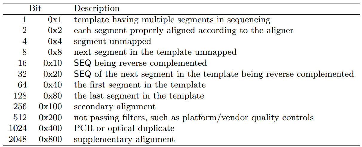
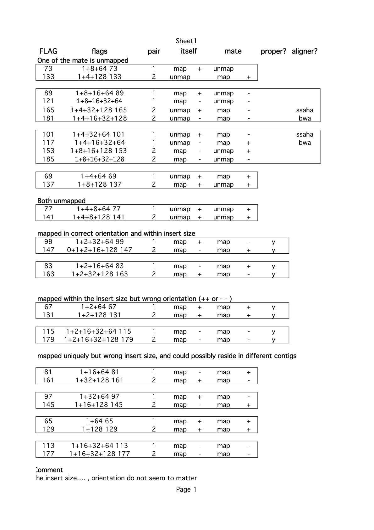
2  FLAG   Bwise FLAG(表明比对类型：pairing，strand，mate strand等)
3  RNAME  比对上的参考序列名,An unmapped segment without coordinate has a ‘*’ at this field. 
4  POS    1-Based的比对上的最左边的定位,POS is set as 0 for an unmapped read without coordinate. If POS is 0, no assumptions can be made about RNAME and CIGAR.
5  MAPQ   比对质量，255表示没有map
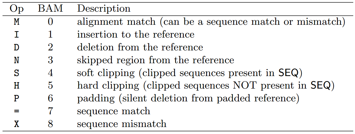
6  CIGAR  Extended CIGAR string (操作符：MIDNSHP) 比对结果信息：匹配碱基数，可变剪接等，*表示不可用。
7  RNEXT   相匹配的另外一条序列，比对上的参考序列名,‘*’ when the information is unavailable, and set as ‘=’ if RNEXT is identical RNAME
8  PNEXT   1-Based leftmost Mate POsition,0 when the information is unavailable.
9  TLEN  插入片段长度,set as 0 for single-segment template or when the information is unavailable
10 SEQ    和参考序列在同一个琏上的比对序列(若比对结果在负意链上，则序列是其反向重复序列), ‘*’ when the sequence is not stored
11 QUAL   比对序列的质量(ASCII-33=Phred base quality),‘*’ when quality is not stored
12 可选的行，以TAG：TYPE：VALUE的形式提供额外的信息

比对区解释

sam/bam比对区包含有此次比对的结果信息，其中主要信息解释如下：

FLAG部分

0x800 表明相应位置的比对属于嵌合体比对；
0x4 没有map上的reads；

CIGAR部分

对于mRNA到基因组的比对，N表示内含子。
More: http://samtools.github.io/hts-specs/SAMv1.pdf

sam文件的几个特例解释

Unmapped reads 统计

Each alignment is one line of the SAM file, but not all lines are successful alignments. Unmapped reads在sam文件中的标记：FLAG列为4而且RNAME列为星号*；

#统计包含星号的比对行数
cut -f3 smallRNA-seq.sam | grep -c \*
#总的比对行数
grep -c -v "^@" smallRNA-seq.sam

How many different read IDs are in the file?

The query (read) ID is in field 1. Some reads may have multiple alignments, so the number of lines is not necessarily the number of reads.

1
2
3

grep -v "@" HR-1B.fq.gz.sam | cut -f1 | sort | uniq | wc -l 
#同时统计此次比对的单端/双端 fa/fq文件发现两者结果不同，说明确实有些reads未能比对上去。
zcat pepper/RNA-seq/sgs-clean-reads/HR-1B.fq.gz | wc -l

How many different read sequences are in the file?

第一列的reads ID仅能表示测序过程中的不同reads，但他们的序列可能因为PCR扩增原因或文库偏好而完全相同，所以统计第10列的uniq序列数能够准确的表示reads总数。

1	cut -f10 smallRNAseq.sam \| sort \| uniq \| wc -l

How many reads are uniquely mapped?

1	cut -f10 smallRNAseq.sam \| sort \| uniq -u \| wc -l

对于 BWA比对结果也可用grep -c XT:A:U smallRNA-seq.sam来准确统计。

How many reads are multi-hits?

1	cut -f1 smallRNA-seq.sam \| sort \| uniq -d \| wc -l

对于 BWA比对结果也可用grep -c XT:A:R smallRNAseq.sam来准确统计。

How many alignments are reported for each read?

1 2	grep -v "^@" smallRNA-seq.sam \| cut -f1 \| sort \| uniq -c \| sort -nr > sortedreadcount.txt grep -v "^@" smallRNA-seq.sam \| cut -f1 \|sort \| uniq -c \| sort -nr \| cut -c1-8 \| sort \| uniq -c

How many different reference sequences are represented in the file?

1	grep -v "^@" smallRNA-seq.sam \| cut –f3 \| sort \| uniq \| wc -l

view

-c 计数
-f 返回指定区间/flags比对结果
-q 返回比对质量大于等于指定值的比对数目
-F 4：统计map 上的 reads总数；
-f 4：统计没有map 上的 reads总数；
To get the unmapped reads from a bam file use :
samtools view -f 4 file.bam > unmapped.sam, the output will be in sam
to get the output in bam use : samtools view -b -f 4 file.bam > unmapped.bam
To get only the mapped reads use the parameter ‘F’, which works like -v of grep and skips the alignments for a specific flag.
samtools view -b -F 4 file.bam > mapped.bam
samtools view -b -F 4 -f 8 file.bam > onlyThisEndMapped.bam
samtools view -b -F 8 -f 4 file.bam > onlyThatEndMapped.bam
samtools view -b -F12 file.bam > bothEndsMapped.bam
samtools merge merged.bam onlyThisEndMapped.bam onlyThatEndMapped.bam bothEndsMapped.bam
对于tophat比对结果：
samtools view -b -f 2 accepted_hits.bam > mappedPairs.bam
Better with:
samtools view -b -f 0x2 accepted_hits.bam > mappedPairs.bam

sort

-m 指定运算内存，支持K，M，G等缩写
-@ 并行运算核数

index

必须对bam文件进行默认情况下的排序后，才能进行index。否则会报错。

建立索引后将产生后缀为.bai的文件，用于快速的随机处理。很多情况下需要有bai文件的存在，特别是显示序列比对情况下。比如samtool的tview命令就需要；gbrowse2显示reads的比对图形的时候也需要。

faidx

对fasta文件建立索引,生成的索引文件以.fai后缀结尾。该命令也能依据索引文件快速提取fasta文件中的某一条（子）序列。
See more： bedtools 使用小结

flagstat

给出BAM文件的比对结果

$ samtools flagstat example.bam
11945742 + 0 in total (QC-passed reads + QC-failed reads)
#总共的reads数
0 + 0 duplicates
7536364 + 0 mapped (63.09%:-nan%)
#总体上reads的匹配率
11945742 + 0 paired in sequencing
#有多少reads是属于paired reads
5972871 + 0 read1
#reads1中的reads数
5972871 + 0 read2
#reads2中的reads数
6412042 + 0 properly paired (53.68%:-nan%)
#完美匹配的reads数：比对到同一条参考序列，并且两条reads之间的距离符合设置的阈值
6899708 + 0 with itself and mate mapped
#paired reads中两条都比对到参考序列上的reads数
636656 + 0 singletons (5.33%:-nan%)
#单独一条匹配到参考序列上的reads数，和上一个相加，则是总的匹配上的reads数。
469868 + 0 with mate mapped to a different chr
#paired reads中两条分别比对到两条不同的参考序列的reads数
243047 + 0 with mate mapped to a different chr (mapQ>=5)

mpileup

samtools还有个非常重要的命令mpileup，以前为pileup。该命令用于生成bcf文件，再使用bcftools进行SNP和Indel的分析。bcftools是samtool中附带的软件，在samtools的安装文件夹中可以找到。
-f 来输入有索引文件的fasta参考序列；
-g 输出到bcf格式。

depth

计算每一个位点或者区域的测序深度；

1	samtools depth sorted.bam > sorted.bam.txt

一共得到3列以指标分隔符分隔的数据，第一列为染色体名称，第二列为位点，第三列为覆盖深度。

贡献来源
http://www.plob.org/2014/01/26/7112.html
http://blog.sina.com.cn/s/blog_670445240101l30k.html
https://www.biostars.org/p/56246/
https://www.biostars.org/p/110039/
https://www.biostars.org/p/95929/
https://www.biostars.org/p/110157/
https://groups.google.com/forum/#!forum/bedtools-discuss
https://code.google.com/p/hydra-sv/

bedtools 使用小结

Posted on 2016-03-18 | In Bioinformatics | Comments: | Views: ℃

| Words count in article: | Reading time ≈

概述

BEDTools是可用于genomic features的比较，相关操作及进行注释的工具。而genomic features通常使用Browser Extensible Data (BED) 或者 General Feature Format (GFF)文件表示，用UCSC Genome Browser进行可视化比较。

与BEDTools使用相关的基本概念

已有的一些genome features信息一般由BED格式或者GFF格式进行存储。
genome features: 功能元素（gene），遗传多态性 (SNPs, INDELs, or structural variants), 已经由测序或者其他方法得到的注释信息，也可以是自定义的一些特征信息。
Overlapping/intersecting features: 两个genome features的区域至少有一个bp的共同片段。

BED和GFF文件的一个差异

BED文件中起始坐标为0，结束坐标至少是1,； GFF中起始坐标是1而结束坐标至少是1。

BEDTools使用总结

intersect/intersectBed：计算 Overlaps

1	bedtools intersect -a A.bed -b B.bed -wa -wb

用来求两个BED或者BAM文件中的overlap，overlap可以进行自定义是整个genome features的overlap还是局部。
默认的结果描述如下图：

加-wa参数可以报告出原始的在A文件中的feature，如下图

加-wb参数可以报告出原始的在B文件中的feature, 加-c参数可以报告出两个文件中的overlap的feature的数量。
当用bedtools intersect 处理大文件时比较耗内存，有效的方法是对A和B文件按照染色体名字(chromosome)和位置(position)排序(sort -k1,1 -k2,2n),然后用-sorted参数重新intersect。

1	bedtools intersect -a A-sorted.bed -b B-sorted.bed --sorted

其他参数：
-wo 返回overlap碱基数

$bedtools  intersect -a A.bed -b B.bed -wo
chr1    0       15      a       chr1    0       4       x       4
chr1    0       15      a       chr1    9       15      z       6
chr1    25      29      b       chr1    18      28      y       3
chr1    18      18      c       chr1    18      28      y       1
chr1    10      14      d       chr1    9       15      z       4
chr1    20      23      e       chr1    18      28      y       3

-v 返回非overlap区间
-s 相同链上的feature
-c 两个文件中的overlap的feature的数量

complement：返回基因组非覆盖区

1	bedtools complement -i <BED/GFF/VCF> -g <genome files>

Slop：增加特征区间大小

要求：单个输入bed文件（-i指定）和genome files

cat ranges-qry.bed 
chr1    0       15      a
chr1    25      29      b
chr1    18      18      c
chr1    10      14      d
chr1    20      23      e
chr1    6       7       f
bedtools slop -i ranges-qry.bed -g genome.txt -b 4
chr1    0       19      a
chr1    21      33      b
chr1    14      22      c
chr1    6       18      d
chr1    16      27      e
chr1    2       11      f
#-b 4	:两端同时缩短4个碱基

-l 3 -r 5:增加左3右5

flank：提取特定区域(启动子区)

要求：基因组GTF文件（-i指定）和genome files

bedtools flank -i mm_GRCm38.75_protein_coding_genes.gtf \
                 -g Mus_musculus.GRCm38_genome.txt \
                 -l 3000 -r 0 > mm_GRCm38_3kb_promoters.gtf
cut -f1,4,5,7 mm_GRCm38_3kb_promoters.gtf | head -n 3
1       3671499 3674498 -
1       4360315 4363314 -
1       4496414 4499413 -

getfasta：提取序列

要求：基因组fasta文件（-fi指定）和提取区间GTF文件(-bed指定)

1 2	bedtools getfasta -fi Mus_musculus.GRCm38.75.dna_rm.toplevel_chr1.fa \ -bed mm_GRCm38_3kb_promoters.gtf -fo mm_GRCm38_3kb_promoters.fasta

-tab Report extract sequences in a tab-delimited format instead of in FASTA format.

提取序列之samtools（速度较快）

#首先建立fai索引文件（第一列为染色体名字，第二列为序列碱基数）
samtools faidx Mus_musculus.GRCm38.75.dna.chromosome.8.fa
#序列提取，多提取区间空格隔开
samtools faidx Mus_musculus.GRCm38.75.dna.chromosome.8.fa \
     8:123407082-123410744 8:123518835-123536649
>8:123407082-123410744
GAGAAAAGCTCCCTTCTTCTCCAGAGTCCCGTCTACCCTGGCTTGGCGAGGGAAAGGAAC
CAGACATATATCAGAGGCAAGTAACCAAGAAGTCTGGAGGTGTTGAGTTTAGGCATGTCT
[...]
>8:123518835-123536649
TCTCGCGAGGATTTGAGAACCAGCACGGGATCTAGTCGGAGTTGCCAGGAGACCGCGCAG
CCTCCTCTGACCAGCGCCCATCCCGGATTAGTGGAAGTGCTGGACTGCTGGCACCATGGT
[...]

nuc: 计算GC含量即各碱基数

1	bedtools nuc -fi hg19.fa -bed CDS.bed

输出结果解释：在原bed文件每行结尾增加以下几列

Output format: 
The following information will be reported after each BED entry:
    1) %AT content
    2) %GC content
    3) Number of As observed
    4) Number of Cs observed
    5) Number of Gs observed
    6) Number of Ts observed
    7) Number of Ns observed
    8) Number of other bases observed
    9) The length of the explored sequence/interval.
    10) The seq. extracted from the FASTA file. (opt., if -seq is used)
    11) The number of times a user's pattern was observed.
        (opt., if -pattern is used.)

genomecov：染色体和全基因组覆盖度计算

要求：单个输入bed文件（-i指定）和genome files；如果输入为bam(-ibam指定)文件，则不需要genome files。

cat ranges-cov-sorted.bed
chr1    4       9
chr1    1       6
chr1    8       19
chr1    25      30
chr2    0       20
$ cat cov.txt
chr1    30
chr2    20
bedtools genomecov -i ranges-cov-sorted.bed -g cov.txt
chr1    0       7       30      0.233333 1
chr1    1       20      30      0.666667
chr1    2       3       30      0.1
chr2    1       20      20      1 2
genome  0       7       50      0.14 3
genome  1       40      50      0.8
genome  2       3       50      0.06
#name 覆盖次数 覆盖碱基数 总碱基数   覆盖度
#同时计算单染色体和全基因组覆盖度

ranges-cov.bed文件需提前排序sort -k1,1 ranges-cov.bed > ranges-cov-sorted.bed

-bg参数可得到每个碱基的覆盖度。

coverage：计算染色体给定区间覆盖度

$ cat A.bed
chr1  0   100
chr1  100 200
chr2  0   100

$ cat B.bed
chr1  10  20
chr1  20  30
chr1  30  40
chr1  100 200

$ bedtools coverage -a A.bed -b B.bed
chr1  0   100  3  30  100 0.3000000
chr1  100 200  1  100 100 1.0000000
chr2  0   100  0  0   100 0.0000000

贡献来源
http://www.plob.org/2012/09/26/3748.html
http://bedtools.readthedocs.org/en/latest/content/bedtools-suite.html
https://code.google.com/archive/p/bedtools/wikis/Usage.wiki
https://code.google.com/archive/p/bedtools/wikis/UsageAdvanced.wiki

R数据整形术之 dplyr

Posted on 2016-03-15 | In R | Comments: | Views: ℃

| Words count in article: | Reading time ≈

数据集类型

将过长过大的数据集转换为显示更友好的 tbl_df 类型:

1	hflights_df <- tbl_df(hflights)

可以 hflights_df 感受一下不再被刷屏的感觉.

基本操作

常用的数据操作行为归纳为以下五种:

筛选: filter()

按给定的逻辑判断筛选出符合要求的子数据集, 类似于 base::subset() 函数

1
2
3

filter(hflights_df, Month == 1, DayofMonth == 1)
#对同一对象的任意个条件组合
filter(hflights_df, Month == 1 | Month == 2)

排列: arrange()

按给定的列名依次对行进行排序

arrange(hflights_df, DayofMonth, Month, Year)
#对列名加 desc() 进行倒序:
arrange(hflights_df, desc(ArrDelay))
#这个函数和 plyr::arrange() 是一样的, 类似于 order()

选择: select()

用列名作参数来选择子数据集:

select(hflights_df, Year, Month, DayOfWeek)
#还可以用 : 来连接列名, 没错, 就是把列名当作数字一样使用
select(hflights_df, Year:DayOfWeek)
用 - 来排除列名:
select(hflights_df, -DrayOfWeek)

变形: mutate()

对已有列进行数据运算并添加为新列:

1	mutate(hflights_df, gain = ArrDelay - DepDelay, speed = Distance / AirTime * 60)

汇总: summarise()

对数据框调用其它函数进行汇总操作, 返回一维的结果:

1	summarise(hflights_df, delay = mean(DepDelay, na.rm = TRUE))

分组动作 group_by()

以上5个动词函数已经很方便了, 但是当它们跟分组操作这个概念结合起来时, 那才叫真正的强大! 当对数据集通过 group_by() 添加了分组信息后,mutate(), arrange() 和 summarise() 函数会自动对这些 tbl 类数据执行分组操作 (R语言泛型函数的优势).

mtfs_df %>%
     group_by(chr) %>%
     summarize(max_recom = max(recom), mean_recom = mean(recom), num=n())

Source: local data frame [23 x 4]
     chr max_recom mean_recom  num
1   chr1   41.5648   2.217759 2095
2  chr10   42.4129   2.162635 1029
3  chr11   36.1703   2.774918  560
[...]

summarise中用到的函数

n(): 计算个数 n_distinct(): 计算 x 中唯一值的个数. (原文为 count_distinct(x))
first(x), last(x) 和 nth(x, n): 返回对应秩的值, 类似于自带函数 x[1], x[length(x)], 和 x[n]

连接符 %>%

使用时把数据名作为开头, 然后依次对此数据进行多步操作.

join功能

两数据集取交，并集等。

inner_join(x,y) 交集
semi_join(x,y)
left_join(x,y)
anti_join(x,y)
inner_join(y,x)
semi_join(y,x)
left_join(y,x)
anti_join(y,x)
full_join(x,y) 并集
【Cheatsheet for dplyr join functions】
深入学习
dplyr 包自带的60页详细文档.
其余几个vignettes (网页) 或 vignette(package = “dplyr”),包含了数据库相关, 混合编程, 运算性能比较, 以及新的 window-functions 等内容.
简单看了下vignette(“window-functions”, package = “dplyr”), 提供了一系列函数, 扩展了原来只能返回一个数值的聚焦类函数(如sum(), mean())至返回等长度的值, 变成 cumsum()和 cummean(), 以及 n(), lead() 和 lag()等便捷功能.
plyr 包的相关文档: 主页
还有data.table包也是很强大的哦, 空下来可以学一学.

R数据整形术之 tidyr

Posted on 2016-03-09 | In R | Comments: | Views: ℃

| Words count in article: | Reading time ≈

Happy families are all alike; every unhappy family is unhappy in its own way — Leo Tolstoy

R数据整形包之一tidyr最近迎来更新(tidyr 0.4.0)，所以有必要对其Tidy data进行学习。
以下为个人简单总结：

#gather--mutate--separate--select--arrange
setwd("F:/Rwork/tidyr")
library(tidyr)

## Warning: package 'tidyr' was built under R version 3.2.3

library(dplyr)

## Warning: package 'dplyr' was built under R version 3.2.2

## 
## Attaching package: 'dplyr'
## 
## The following objects are masked from 'package:stats':
## 
##     filter, lag
## 
## The following objects are masked from 'package:base':
## 
##     intersect, setdiff, setequal, union

preg <-read.csv("preg.csv",stringsAsFactors = FALSE)
preg

##           name treatmenta treatmentb
## 1   John Smith         NA         18
## 2     Jane Doe          4          1
## 3 Mary Johnson          6          7

preg6 <-tbl_df(read.csv("preg.csv",stringsAsFactors = FALSE))
preg6

## Source: local data frame [3 x 3]
## 
##           name treatmenta treatmentb
##          (chr)      (int)      (int)
## 1   John Smith         NA         18
## 2     Jane Doe          4          1
## 3 Mary Johnson          6          7

preg2<-preg %>% 
  gather(treatment,n,treatmenta:treatmentb) %>%  
#The first argument, is the name of the key column, which is the name of the variable defined by the values of the column headings. 
#The second argument is the name of the value column.
#The third argument defines the columns to gather, here, every column except religion.
 #gather(treatment,n,-name,na.rm = TRUE)    #the same above # na.rm to drop any missing values from the gather columns
  mutate(treatment=gsub("treatment","",treatment)) %>%
  arrange(name,treatment)   #arrange=sort
preg2

##           name treatment  n
## 1     Jane Doe         a  4
## 2     Jane Doe         b  1
## 3   John Smith         a NA
## 4   John Smith         b 18
## 5 Mary Johnson         a  6
## 6 Mary Johnson         b  7

#each deplay one by one 
preg3<-preg %>% 
  gather(treatment,n,treatmenta:treatmentb)
preg3

##           name  treatment  n
## 1   John Smith treatmenta NA
## 2     Jane Doe treatmenta  4
## 3 Mary Johnson treatmenta  6
## 4   John Smith treatmentb 18
## 5     Jane Doe treatmentb  1
## 6 Mary Johnson treatmentb  7

preg33<-preg3 %>% separate(treatment, c("Treatments", "group"),9 )  #separate
preg33

##           name Treatments group  n
## 1   John Smith  treatment     a NA
## 2     Jane Doe  treatment     a  4
## 3 Mary Johnson  treatment     a  6
## 4   John Smith  treatment     b 18
## 5     Jane Doe  treatment     b  1
## 6 Mary Johnson  treatment     b  7

preg333<-preg33 %>% select(name,group,n)  # select
preg333

##           name group  n
## 1   John Smith     a NA
## 2     Jane Doe     a  4
## 3 Mary Johnson     a  6
## 4   John Smith     b 18
## 5     Jane Doe     b  1
## 6 Mary Johnson     b  7

preg3333<-preg333 %>% spread(group,n)  #spread: one column become two column
preg3333

##           name  a  b
## 1     Jane Doe  4  1
## 2   John Smith NA 18
## 3 Mary Johnson  6  7

preg4<-preg3 %>% mutate(treatment=gsub("treatment","",treatment))
preg4

##           name treatment  n
## 1   John Smith         a NA
## 2     Jane Doe         a  4
## 3 Mary Johnson         a  6
## 4   John Smith         b 18
## 5     Jane Doe         b  1
## 6 Mary Johnson         b  7

preg5<-preg4 %>% arrange(name,treatment)
preg5

##           name treatment  n
## 1     Jane Doe         a  4
## 2     Jane Doe         b  1
## 3   John Smith         a NA
## 4   John Smith         b 18
## 5 Mary Johnson         a  6
## 6 Mary Johnson         b  7

#reads all files from the same locaed pathway  into a single data frame.
library(plyr)

## -------------------------------------------------------------------------
## You have loaded plyr after dplyr - this is likely to cause problems.
## If you need functions from both plyr and dplyr, please load plyr first, then dplyr:
## library(plyr); library(dplyr)
## -------------------------------------------------------------------------
## 
## Attaching package: 'plyr'
## 
## The following objects are masked from 'package:dplyr':
## 
##     arrange, count, desc, failwith, id, mutate, rename, summarise,
##     summarize

paths <- dir("F:/Rwork/tidyr", pattern = "\\.csv$", full.names = TRUE)
names(paths) <- basename(paths)
all<-ldply(paths, read.csv, stringsAsFactors = FALSE)
all

##               .id         name treatmenta treatmentb
## 1 preg - Copy.csv   John Smith         NA         18
## 2 preg - Copy.csv     Jane Doe          4          1
## 3 preg - Copy.csv Mary Johnson          6          7
## 4        preg.csv   John Smith         NA         18
## 5        preg.csv     Jane Doe          4          1
## 6        preg.csv Mary Johnson          6          7

#get some data from name column incloud John Smith and Jane Doe  located in preg3 data frame 
subset(preg3, name %in% c("John Smith", "Jane Doe"))

##         name  treatment  n
## 1 John Smith treatmenta NA
## 2   Jane Doe treatmenta  4
## 4 John Smith treatmentb 18
## 5   Jane Doe treatmentb  1

Economist_Graph：复杂图形修改

Posted on 2016-03-09 | In R | Comments: | Views: ℃

| Words count in article: | Reading time ≈

原图：http://www.economist.com/node/21541178

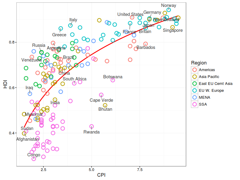
Basic plot

library(ggplot2)
dat <- read.csv("EconomistData.csv")
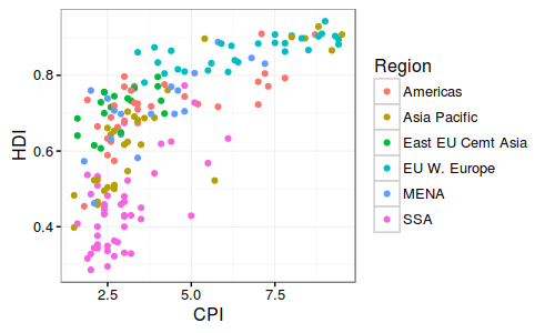
pc1 <- ggplot(dat, aes(x = CPI, y = HDI, color = Region))+
       geom_point()

Trend line

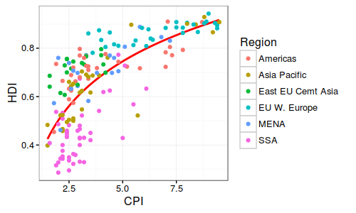
pc2 <- pc1 +
   geom_smooth(aes(group = 1),
               method = "lm",
               formula = y ~ log(x),
               se = FALSE,
               color = "red") +
   geom_line()

Open points

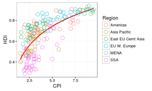
1 2	pc3 <- pc2 + geom_point(shape = 1, size = 4)

Labelling points

pointsToLabel <- c("Russia", "Venezuela", "Iraq", "Myanmar", "Sudan",
                   "Afghanistan", "Congo", "Greece", "Argentina", "Brazil",
                   "India", "Italy", "China", "South Africa", "Spane",
                   "Botswana", "Cape Verde", "Bhutan", "Rwanda", "France",
                   "United States", "Germany", "Britain", "Barbados", "Norway", "Japan",
                   "New Zealand", "Singapore")
library("ggrepel")
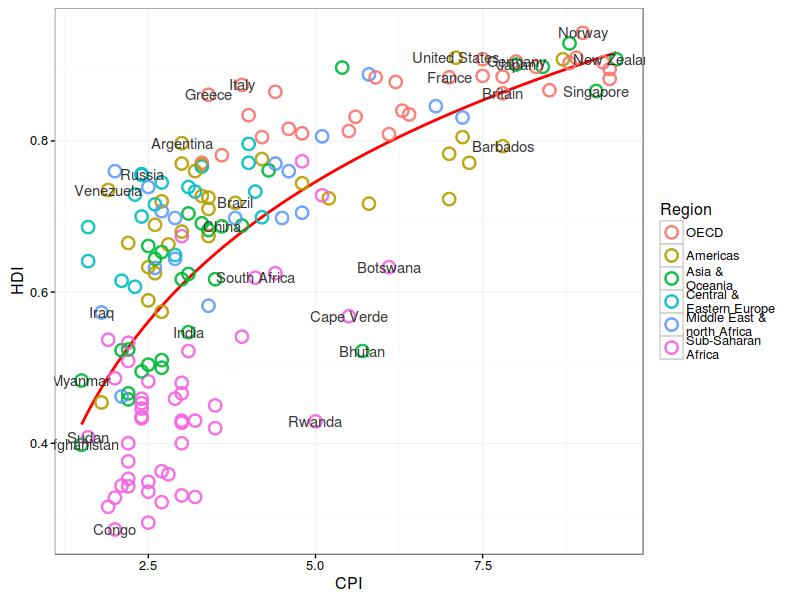
pc4 <- pc3 +  geom_text_repel(aes(label = Country),
            color = "gray20",
            data = subset(dat, Country %in% pointsToLabel),
            force = 10)

选择性的标注想要的点

Change the region labels and order

dat$Region <- factor(dat$Region,
                     levels = c("EU W. Europe",
                                "Americas",
                                "Asia Pacific",
                                "East EU Cemt Asia",
                                "MENA",
                                "SSA"),
                     labels = c("OECD",
                                "Americas",
                                "Asia &\nOceania",
                                "Central &\nEastern Europe",
                                "Middle East &\nnorth Africa",
                                "Sub-Saharan\nAfrica"))
pc4$data <- dat
pc4

修改图例值和顺序

Add title and format axes

library(grid)
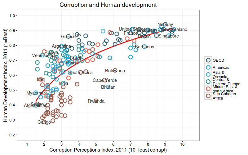
pc5 <- pc4 +
  scale_x_continuous(name = "Corruption Perceptions Index, 2011 (10=least corrupt)",
                     limits = c(.9, 10.5),
                     breaks = 1:10) +
  scale_y_continuous(name = "Human Development Index, 2011 (1=Best)",
                     limits = c(0.2, 1.0),
                     breaks = seq(0.2, 1.0, by = 0.1)) +
  scale_color_manual(name = "",
                     values = c("#24576D",
                                "#099DD7",
                                "#28AADC",
                                "#248E84",
                                "#F2583F",
                                "#96503F")) +
  ggtitle("Corruption and Human development"))

利用scale来修改x，y轴，颜色和标出title

Theme tweaks

library(grid) # for the 'unit' function
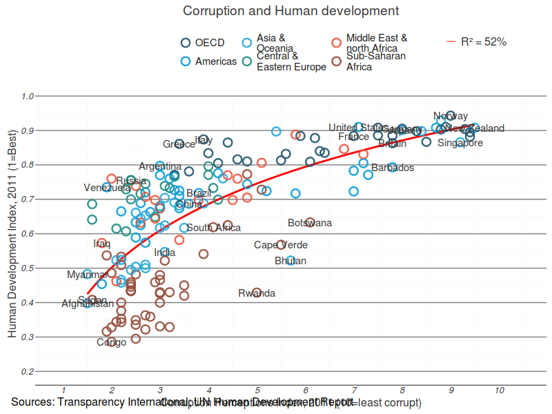
pc6 <- pc5 +
  theme_minimal() + # start with a minimal theme and add what we need
  theme(text = element_text(color = "gray20"),
        legend.position = c("top"), # position the legend in the upper left 
        legend.direction = "horizontal",
        legend.justification = 0.1, # anchor point for legend.position.
        legend.text = element_text(size = 11, color = "gray10"),
        axis.text = element_text(face = "italic"),
        axis.title.x = element_text(vjust = -1), # move title away from axis
        axis.title.y = element_text(vjust = 2), # move away for axis
        axis.ticks.y = element_blank(), # element_blank() is how we remove elements
        axis.line = element_line(color = "gray40", size = 0.5),
        axis.line.y = element_blank(),
        panel.grid.major = element_line(color = "gray50", size = 0.5),
        panel.grid.major.x = element_blank()
        ))

微调主题

Add model R^2 and source note

mR2 <- summary(lm(HDI ~ log(CPI), data = dat))$r.squared
library(grid)
png(file = "images/econScatter10.png", width = 800, height = 600)
pc6 
grid.text("Sources: Transparency International; UN Human Development Report",
         x = .02, y = .03,
         just = "left",
         draw = TRUE)
grid.segments(x0 = 0.81, x1 = 0.825,
              y0 = 0.90, y1 = 0.90,
              gp = gpar(col = "red"),
              draw = TRUE)
grid.text(paste0("R² = ",
                 as.integer(mR2*100),
                 "%"),
          x = 0.835, y = 0.90,
          gp = gpar(col = "gray20"),
          draw = TRUE,
          just = "left")

dev.off()

Contribution from ：
http://tutorials.iq.harvard.edu/R/Rgraphics/Rgraphics.html

myself ggplot2 learning tip (再学ggplot2：遗漏细节)

Posted on 2016-03-09 | In R | Comments: | Views: ℃

| Words count in article: | Reading time ≈

原图：http://www.economist.com/node/21541178

ggplot2绘图语法结构：

ggplot(data = <default data set>, 
       aes(x = <default x axis variable>,
           y = <default y axis variable>,
           ... <other default aesthetic mappings>),
       ... <other plot defaults>) +

       geom_<geom type>(aes(size = <size variable for this geom>, 
                      ... <other aesthetic mappings>),
                  data = <data for this point geom>,
                  stat = <statistic string or function>,
                  position = <position string or function>,
                  color = <"fixed color specification">,
                  <other arguments, possibly passed to the _stat_ function) +

  scale_<aesthetic>_<type>(name = <"scale label">,
                     breaks = <where to put tick marks>,
                     labels = <labels for tick marks>,
                     ... <other options for the scale>) +

  theme(plot.background = element_rect(fill = "gray"),
        ... <other theme elements>)

Geometric Objects(geom_XX) and Aesthetics (aes())

1	geom_<tab>查看所有Geometric Objects（几何学对象）

Statistical Transformations（统计变换）

统计变换（stat_）比如求均值，求方差等，当我们需要展示出某个变量的某种统计特征的时候，需要用到统计变换。
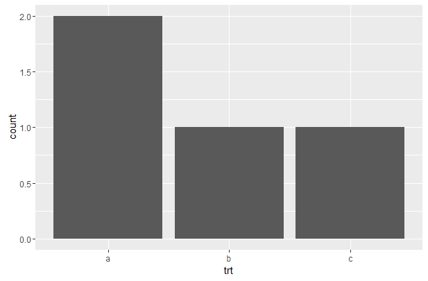
每一个geom_XX都有一个默认的统计量，可通过args(geom_XX)查看（args(stat_bin)）例如geom_bar的默认统计量是stat_count,表示进行计数。什么意思呢？举例如下：

> library(ggplot2)
> df <- data.frame(trt = c("a","a", "b", "c"), outcome = c(2.3,5, 1.9, 3.2))
> df
  trt outcome
1   a     2.3
2   a     5.0
3   b     1.9
4   c     3.2
> ##stat()
> ggplot(df, aes(trt, outcome)) +
  geom_bar()
Error: stat_count() must not be used with a y aesthetic.
#成功报错，因为第一句aes()中我们指定了y轴为outcome，即一个x轴的trt值对应一个y轴的outcome值，而geom_bar()
#中stat_count要进行计数，即计数trt中相同值出现的次数.最终y轴指定的outcome与需要表示的count值冲突，报错。
##解决：
> ggplot(df, aes(trt)) +
  geom_bar()

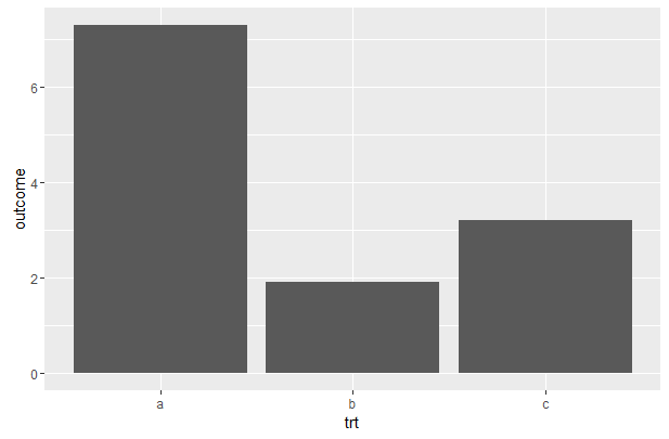
如果想要表示相同trt值相加后的对应值，修改stat=indentity即可。

1 2	> ggplot(df, aes(trt, outcome)) + + geom_bar(stat = "identity")

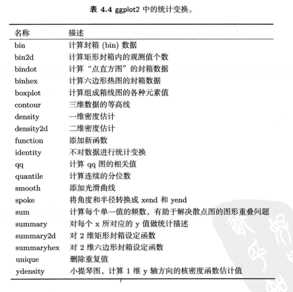
ggplot2中包含的统计变换有如下多种：

更多参见：https://www.zhihu.com/question/24779017

Scales

控制`aes()`映射

Aesthetic (aes()) 映射仅仅是告诉一个变量应该映射到一个aesthetic，但并没有说明如何映射？例如，当我们用aes(shape=x)去映射一个变量到shape时，并没有说明用什么shape；同样的，aes(color=z)并无说明用什么颜色；通常在我们未定义这些时ggplot2会自动用默认值，而我们可以通过scale来修改这些值。
在ggplot2中scales包括：

position

color and fill

size

shape

line type

x,y

### 修改方式

1 2	scale_<aesthetic>_<type>(name,limits,breaks,labels) 通过键入scale_<tab>查看全部可修改函数。

特殊scale函数有额外参数，例如对颜色的修改scale_color_continuous函数有low和high参数。

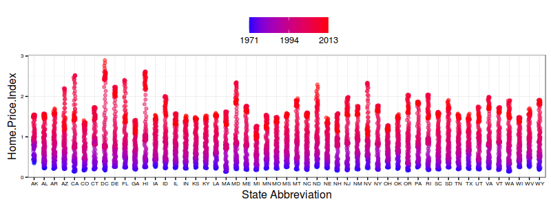
scale_x_discrete(name="State Abbreviation") +
scale_color_continuous(name="",
                         breaks = c(19751, 19941, 20131),
                         labels = c(1971, 1994, 2013),
                         low = "blue", high = "red")

## Faceting
### 分面: 一页多图
facet_wrap()：对数据分类只能应用一个标准，例facet_wrap(~State, ncol = 10)),按State分组后每行设置10个小图依次画出全部。
facet_grid()：多个标准对数据进行分组绘图,facet_grid(color~cut，margins=TRUE)，波浪号前为小图分行标准，后面为分列标准，margins指用于分面的包含每个变量元素所有数据的数据组，相当于每个小图一个title。
## Themes
### 主题
更多ggplot2主题演示如下：
http://docs.ggplot2.org/dev/vignettes/themes.html
https://github.com/jrnold/ggthemes
### 修改主题默认值

1 2	theme_minimal() + theme(text = element_text(color = "turquoise"))

### 自定义主题

theme_new <- theme_bw() +
  theme(plot.background = element_rect(size = 1, color = "blue", fill = "black"),
        text=element_text(size = 12, family = "Serif", color = "ivory"),
        axis.text.y = element_text(colour = "purple"),
        axis.text.x = element_text(colour = "red"),
        panel.background = element_rect(fill = "pink"),
        strip.background = element_rect(fill = muted("orange")))

p5 + theme_new

## 关于晕晕的aes()

任何与数据向量顺序相关，需要逐个指定的参数都必须写在aes里

什么？还是搞不清该放aes里面还是外面？那就记着想统一整个图层时就放到aes外，想分成不同组调整，并且已经有一个与x、y长度一致的分组变量了，那就放到aes里

##其他总结

加注释，所有注释的实现都是通过annotate函数实现的，geom_text()是兼职的。

theme函数最妙的地方是将对于数据相关的美学调整和与数据无关的美学调整分离，将数据处理与数据美学分开，数据美学与数据无关的调整分开。

Noncoding RNAs (ncRNAs)

Posted on 2016-01-29 | In molecular biology | Comments: | Views: ℃

| Words count in article: | Reading time ≈

Noncoding RNAs (ncRNAs)

most ncRNAs operate as RNA-protein complexes, including ribosomes, snRNPs, snoRNPs, telomerase, microRNAs, and long ncRNAs.

Non-coding RNA database

http://research.imb.uq.edu.au/rnadb/

tiramisutes

hope bioinformatics blog

RSS

GitHub E-Mail Weibo Twitter

Summary Statistics

mean(),max(),min(),range()，sd()

quantile(),fivenum()，IQR()

summary()

Statistical Tests

Comparing means

Comparing paired data(means)

Comparing variances of two populations

Comparing means across more than two groups

Correlation tests

SQLite数据库整体查询命令

dot-commands

SQLite数据类型

数据库内容查询

万能的SELECT命令

集合函数（Aggregate）

行分组(GROUP BY)

自己动手写数据库

创建tables

数据写入table

建立索引

修改/删除table

python中交互操作SQLite

连接SQLite数据库并创建table

数据载入table

直接删除

打印删除rm命令并检查

将删除文件放入临时文件夹（tmp）

sam文件格式

比对区解释

sam文件的几个特例解释

Unmapped reads 统计

How many different read IDs are in the file?

How many different read sequences are in the file?

How many reads are uniquely mapped?

How many reads are multi-hits?

How many alignments are reported for each read?

How many different reference sequences are represented in the file?

view

sort

index

faidx

flagstat

mpileup

depth

概述

与BEDTools使用相关的基本概念

BED和GFF文件的一个差异

相关格式

BED format

GFF format

genome files

BEDTools使用总结

intersect/intersectBed：计算 Overlaps

complement：返回基因组非覆盖区

Slop：增加特征区间大小

flank：提取特定区域(启动子区)

getfasta：提取序列

nuc: 计算GC含量即各碱基数

genomecov：染色体和全基因组覆盖度计算

coverage：计算染色体给定区间覆盖度

数据集类型

基本操作

筛选: filter()

排列: arrange()

选择: select()

变形: mutate()

汇总: summarise()

分组动作 group_by()

连接符 %>%

join功能

深入学习

Basic plot

Trend line

Open points

Labelling points

Change the region labels and order

Add title and format axes

Theme tweaks

Add model R^2 and source note

控制`aes()`映射