学习WGCNA总结

在转录组数据处理过程中我们经常会用到差异表达分析这一概念，通过比较不同处理或不同组织间基因表达量(FPKM)差异来寻找特异基因，但这前提是你的不同处理或不同组织样本较少，当不同处理或组织有较多样本，如40个，此时的两两比较有780组比较^_^,这根本不是我们想要的结果；

此时就需要WGCNA(weighted gene co-expression network analysis)将复杂的数据进行归纳整理。除了这种最常见的比较差异表达，我们还想知道在不同处理或不同组织间是否有些基因的表达存在内在的联系或相关性？WGCNA同样可以帮助我们预测基因间的相互作用关系。

WGCNA is based on correlation and not differential expression comparisons.

WGCNA术语

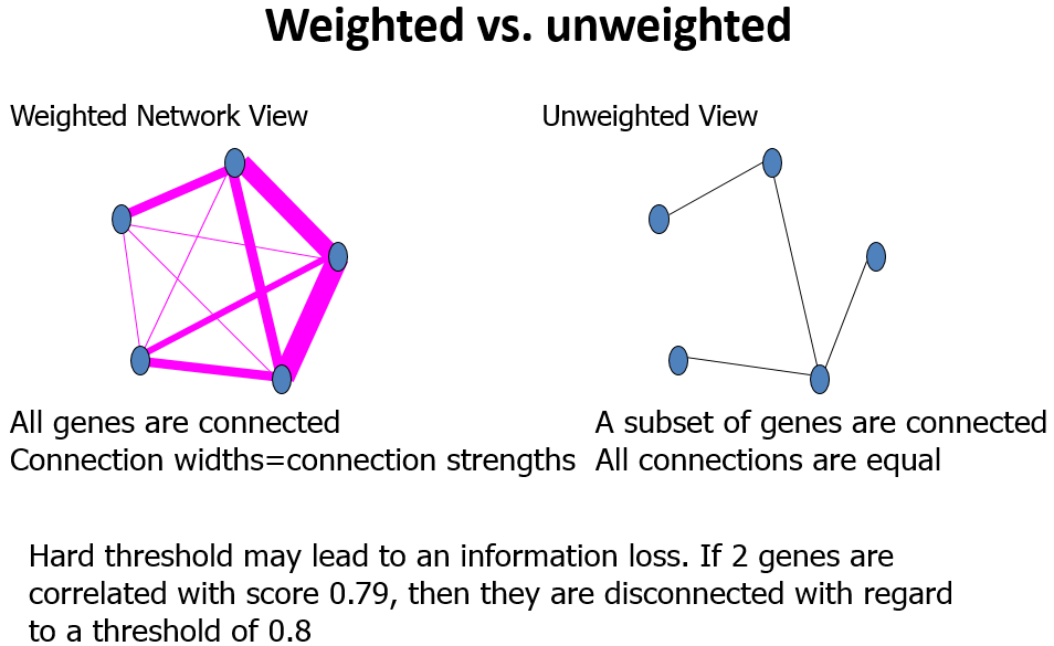
权重(weghted)

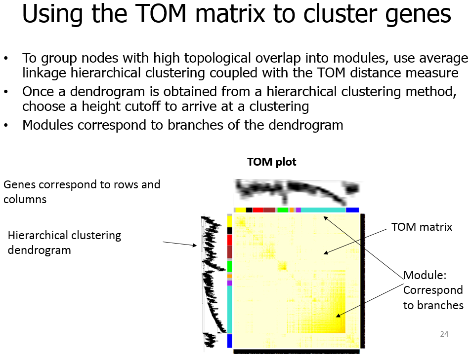
Module

模块(module)：表达模式相似的基因分为一类，这样的一类基因成为模块；

Eigengene

Eigengene（eigen- +‎ gene）：基因和样本构成的矩阵，https://en.wiktionary.org/wiki/eigengene；

Adjacency Matrix

邻近矩阵：是图的一种存储形式，用一个一维数组存放图中所有顶点数据；用一个二维数组存放顶点间关系（边或弧）的数据，这个二维数组称为邻接矩阵；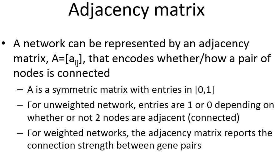

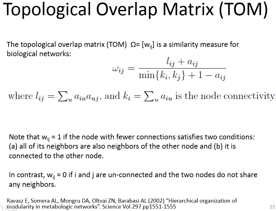
Topological Overlap Matrix(TOM)

整体思路

先对数据进行处理→分层聚类→表达模式相似的基因组成模块→研究某一个模块中相关基因的功能富集(GO,KEGG)，各个模块与样本表型数据间的相关性，各个模块与样本本身间的相关性(没有表型数据的情况，如不同组织)→具体到特定模块后分析其所包含基因间的相互作用网络关系，并找出其中的关键基因。

分析构建的网络寻找以下有用信息

这类处于调控网络中心的基因称为核心基因（hub gene），这类基因通常是转录因子等关键的调控因子，是值得我们优先深入分析和挖掘的对象。

在网络中，被调控线连接的基因，其表达模式是相似的。那么它们潜在有相似的功能。所以，在这个网络中，如果线条一端的基因功能是已知的，那么就可以预测线条另一端的功能未知的基因也有相似的功能。

R脚本

输入数据为RNA-seq不同处理或组织所有样本的FPKM值组成的矩阵，切记含有 0 的要去掉；

setwd("F:/WGCNA")
library(WGCNA)
options(stringsAsFactors = FALSE)
enableWGCNAThreads()
#############################################################################
####################### 一、 数据读入，处理和保存 ##############################
#############################################################################
fpkm<- read.csv("trans_counts.counts.matrix.TMM_normalized.FPKM.nozero.csv")
#~~~~~~~~~~~~~~~~~~
head(fpkm)
   GeneID PN_1_TPM PN_1_07_TPM PN_1_08_TPM PN_2_TPM PN_2_09_TPM PN_2_10_TPM
1 MSTRG.1 0.000000    1.456143    1.093308 0.204315    0.000000    0.000000
2 MSTRG.2 1.516181    0.849313    2.010783 1.567867    2.045446    2.246402
3 MSTRG.3 1.305084    1.207246    0.889166 1.470162    0.340003    0.421222
4 MSTRG.4 2.744250    2.791988    2.500786 2.719017    1.954149    2.468110
5 MSTRG.5 1.946825    1.470012    1.263171 0.205806    1.644505    1.638583
6 MSTRG.6 1.325277    0.793530    1.932236 1.210156    1.834274    2.153466
#~~~~~~~~~~~~~~~~~~
dim(fpkm)
names(fpkm)
datExpr0=as.data.frame(t(fpkm[,-c(1)]));
names(datExpr0)=fpkm$trans;
rownames(datExpr0)=names(fpkm)[-c(1)];
#data<-log10(date[,-1]+0.01)
# *************************************************************
# 检测输入基因是否含有缺失值,并处理 ******************************
# *************************************************************
gsg = goodSamplesGenes(datExpr0, verbose = 3);
gsg$allOK
#~~~~~~~~~~~~~~~~~~
# 如果上一步返回TRUE则跳过此步，如果返回FALSE则执行如下if语句去掉存在较多缺失值的基因所在行
if (!gsg$allOK)
{
  # Optionally, print the gene and sample names that were removed:
  if (sum(!gsg$goodGenes)>0)
    printFlush(paste("Removing genes:", paste(names(datExpr0)[!gsg$goodGenes], collapse = ", ")));
  if (sum(!gsg$goodSamples)>0)
    printFlush(paste("Removing samples:", paste(rownames(datExpr0)[!gsg$goodSamples], collapse = ", ")));
# Remove the offending genes and samples from the data:
datExpr0 = datExpr0[gsg$goodSamples, gsg$goodGenes]
}
# 再次检测
dim(datExpr0)
gsg = goodSamplesGenes(datExpr0, verbose = 3);
gsg$allOK
#~~~~~~~~~~~~~~~~~~
# ***************************************************************
# 聚类检测输入样本是否含有异常值（obvious outliers）,并处理 ********
# ***************************************************************
sampleTree = hclust(dist(datExpr0), method = "average")
#sizeGrWindow(12,9)
par(cex = 0.6)
par(mar = c(0,4,2,0))
plot(sampleTree, main = "Sample clustering to detect outliers", sub="", xlab="", cex.lab = 1.5,
     cex.axis = 1.5, cex.main = 2)
abline(h = 80000, col = "red");
clust = cutreeStatic(sampleTree, cutHeight = 80000, minSize = 10)
table(clust)
keepSamples = (clust==1)
datExpr = datExpr0[keepSamples, ]
nGenes = ncol(datExpr)
nSamples = nrow(datExpr)
save(datExpr, file = "AS-green-FPKM-01-dataInput.RData")
#############################################################################
############################ 二、 选择合适的阀值 ##############################
#############################################################################
powers = c(c(1:10), seq(from = 12, to=20, by=2))
# Call the network topology analysis function
sft = pickSoftThreshold(datExpr, powerVector = powers, verbose = 5)
# Plot the results:
##sizeGrWindow(9, 5)
par(mfrow = c(1,2));
cex1 = 0.9;
# Scale-free topology fit index as a function of the soft-thresholding power
plot(sft$fitIndices[,1], -sign(sft$fitIndices[,3])*sft$fitIndices[,2],
     xlab="Soft Threshold (power)",ylab="Scale Free Topology Model Fit,signed R^2",type="n",
     main = paste("Scale independence"));
text(sft$fitIndices[,1], -sign(sft$fitIndices[,3])*sft$fitIndices[,2],
     labels=powers,cex=cex1,col="red");
# this line corresponds to using an R^2 cut-off of h
abline(h=0.90,col="red")
# Mean connectivity as a function of the soft-thresholding power
plot(sft$fitIndices[,1], sft$fitIndices[,5],
     xlab="Soft Threshold (power)",ylab="Mean Connectivity", type="n",
     main = paste("Mean connectivity"))
text(sft$fitIndices[,1], sft$fitIndices[,5], labels=powers, cex=cex1,col="red")

#############################################################################
############################ 三、 网络构建和可视化 #############################
#############################################################################
#=====================================================================================
#=====================================================================================
# 网络构建有两种方法，One-step和Step-by-step；
# 第一种：一步法进行网络构建
#=====================================================================================
#=====================================================================================

################################################################################
### 3.1 一步法网络构建：One-step network construction and module detection ######
#3.1.1. 网络构建 ###############################################################
###############################################################################
dim(datExpr)
net = blockwiseModules(datExpr, power = 6, maxBlockSize = 6000,
                       TOMType = "unsigned", minModuleSize = 30,
                       reassignThreshold = 0, mergeCutHeight = 0.25,
                       numericLabels = TRUE, pamRespectsDendro = FALSE,
                       saveTOMs = TRUE,
                       saveTOMFileBase = "AS-green-FPKM-TOM",
                       verbose = 3)
table(net$colors)
###############################################################################
#3.1.2. 绘画结果展示 ###########################################################
###############################################################################
# open a graphics window
#sizeGrWindow(12, 9)
# Convert labels to colors for plotting
mergedColors = labels2colors(net$colors)
# Plot the dendrogram and the module colors underneath
plotDendroAndColors(net$dendrograms[[1]], mergedColors[net$blockGenes[[1]]],
                    "Module colors",
                    dendroLabels = FALSE, hang = 0.03,
                    addGuide = TRUE, guideHang = 0.05)
###############################################################################
#3.1.3. 结果保存 ###############################################################
###############################################################################                  
moduleLabels = net$colors
moduleColors = labels2colors(net$colors)
table(moduleColors)
MEs = net$MEs;
geneTree = net$dendrograms[[1]];
save(MEs, moduleLabels, moduleColors, geneTree,
     file = "AS-green-FPKM-02-networkConstruction-auto.RData")
###############################################################################
#3.1.4. 导出网络到 Cytoscape ###################################################
###############################################################################  
# Recalculate topological overlap if needed
TOM = TOMsimilarityFromExpr(datExpr, power = 6);
# Read in the annotation file
# annot = read.csv(file = "GeneAnnotation.csv");
# Select modules需要修改，根据table(moduleColors)的结果选择需要导出的模块颜色
modules = c("turquoise", "blue");
# Select module probes选择模块探测
probes = names(datExpr)
inModule = is.finite(match(moduleColors, modules));
modProbes = probes[inModule];
#modGenes = annot$gene_symbol[match(modProbes, annot$substanceBXH)];
# Select the corresponding Topological Overlap
modTOM = TOM[inModule, inModule];
dimnames(modTOM) = list(modProbes, modProbes)
# Export the network into edge and node list files Cytoscape can read
cyt = exportNetworkToCytoscape(modTOM,
                               edgeFile = paste("AS-green-FPKM-One-step-CytoscapeInput-edges-", paste(modules, collapse="-"), ".txt", sep=""),
                               nodeFile = paste("AS-green-FPKM-One-step-CytoscapeInput-nodes-", paste(modules, collapse="-"), ".txt", sep=""),
                               weighted = TRUE,
                               threshold = 0.02,
                               nodeNames = modProbes,
                               #altNodeNames = modGenes,
                               nodeAttr = moduleColors[inModule]);
#################################################################################################
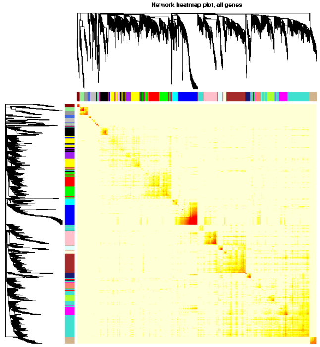
#3.1.5. 分析网络可视化，用heatmap可视化权重网络，heatmap每一行或列对应一个基因，颜色越深表示有较高的邻近
#################################################################################################
options(stringsAsFactors = FALSE);
lnames = load(file = "AS-green-FPKM-01-dataInput.RData");
lnames
lnames = load(file = "AS-green-FPKM-02-networkConstruction-auto.RData");
lnames
nGenes = ncol(datExpr)
nSamples = nrow(datExpr)
#====================================
#3.1.5.1. 可视化全部基因网络 ==========
#====================================
# Calculate topological overlap anew: this could be done more efficiently by saving the TOM
# calculated during module detection, but let us do it again here.
dissTOM = 1-TOMsimilarityFromExpr(datExpr, power = 6);
# Transform dissTOM with a power to make moderately strong connections more visible in the heatmap
plotTOM = dissTOM^7;
# Set diagonal to NA for a nicer plot
diag(plotTOM) = NA;
# Call the plot function
#sizeGrWindow(9,9)
TOMplot(plotTOM, geneTree, moduleColors, main = "Network heatmap plot, all genes")
#====================================
#3.1.5.2. 随便选取1000个基因来可视化 ==
#====================================
nSelect = 1000
# For reproducibility, we set the random seed
set.seed(10);
select = sample(nGenes, size = nSelect);
selectTOM = dissTOM[select, select];
# There's no simple way of restricting a clustering tree to a subset of genes, so we must re-cluster.
selectTree = hclust(as.dist(selectTOM), method = "average")
selectColors = moduleColors[select];
# Open a graphical window
#sizeGrWindow(9,9)
# Taking the dissimilarity to a power, say 10, makes the plot more informative by effectively changing
# the color palette; setting the diagonal to NA also improves the clarity of the plot
plotDiss = selectTOM^7;
diag(plotDiss) = NA;
TOMplot(plotDiss, selectTree, selectColors, main = "Network heatmap plot, selected genes")
#=====================================================================================
#=====================================================================================
#  第二种：一步步的进行网络构建
#=====================================================================================
#=====================================================================================

###############################################################################
### 3.2 Step-by-step network construction and module detection ################
###############################################################################
#2.选择合适的阀值，同上
###############################################################################
#3.2.1. 网络构建 ###############################################################
###############################################################################
#~~~~~~~~~~~~~~~~~~~~~~~~~~~~~~~~~~~~~~~~~~~~~~~~~~~~~~~~~~~~~~~~~~~~~~~~~
# (1) Co-expression similarity and adjacency ~~~~~~~~~~~~~~~~~~~~~~~~~~~~~
#~~~~~~~~~~~~~~~~~~~~~~~~~~~~~~~~~~~~~~~~~~~~~~~~~~~~~~~~~~~~~~~~~~~~~~~~~
softPower = 6;
adjacency = adjacency(datExpr, power = softPower);
#~~~~~~~~~~~~~~~~~~~~~~~~~~~~~~~~~~~~~~~~~~~~~~~~~~~~~~~~~~~~~~~~~~~~~~~~~
#(2) 邻近矩阵到拓扑矩阵的转换，Turn adjacency into topological overlap ~~~~~
#~~~~~~~~~~~~~~~~~~~~~~~~~~~~~~~~~~~~~~~~~~~~~~~~~~~~~~~~~~~~~~~~~~~~~~~~~
TOM = TOMsimilarity(adjacency);
dissTOM = 1-TOM
#~~~~~~~~~~~~~~~~~~~~~~~~~~~~~~~~~~~~~~~~~~~~~~~~~~~~~~~~~~~~~~~~~~~~~~~~~
# (3) 聚类拓扑矩阵  ~~~~~~~~~~~~~~~~~~~~~~~~~~~~~~~~~~~~~~~~~~~~~~~~~~~~~~~
#~~~~~~~~~~~~~~~~~~~~~~~~~~~~~~~~~~~~~~~~~~~~~~~~~~~~~~~~~~~~~~~~~~~~~~~~~
#Call the hierarchical clustering function
geneTree = hclust(as.dist(dissTOM), method = "average");
# Plot the resulting clustering tree (dendrogram)
#sizeGrWindow(12,9)
plot(geneTree, xlab="", sub="", main = "Gene clustering on TOM-based dissimilarity",
     labels = FALSE, hang = 0.04);
#~~~~~~~~~~~~~~~~~~~~~~~~~~~~~~~~~~~~~~~~~~~~~~~~~~~~~~~~~~~~~~~~~~~~~~~~~
#(4) 聚类分支的休整dynamicTreeCut ~~~~~~~~~~~~~~~~~~~~~~~~~~~~~~~~~~~~~~~~~
#~~~~~~~~~~~~~~~~~~~~~~~~~~~~~~~~~~~~~~~~~~~~~~~~~~~~~~~~~~~~~~~~~~~~~~~~~
# We like large modules, so we set the minimum module size relatively high:
minModuleSize = 30;
# Module identification using dynamic tree cut:
dynamicMods = cutreeDynamic(dendro = geneTree, distM = dissTOM,
                            deepSplit = 2, pamRespectsDendro = FALSE,
                            minClusterSize = minModuleSize);
table(dynamicMods)
###############################################################################
#3.2.2. 绘画结果展示 ###########################################################
###############################################################################
# Convert numeric lables into colors
dynamicColors = labels2colors(dynamicMods)
table(dynamicColors)
# Plot the dendrogram and colors underneath
#sizeGrWindow(8,6)
plotDendroAndColors(geneTree, dynamicColors, "Dynamic Tree Cut",
                    dendroLabels = FALSE, hang = 0.03,
                    addGuide = TRUE, guideHang = 0.05,
                    main = "Gene dendrogram and module colors")
###############################################################################
#3.2.3. 聚类结果相似模块的融合，Merging of modules whose expression profiles are very similar
###############################################################################
#在聚类树中每一leaf是一个短线，代表一个基因，
#不同分之间靠的越近表示有高的共表达基因，将共表达极其相似的modules进行融合
###############################################################################
# Calculate eigengenes
MEList = moduleEigengenes(datExpr, colors = dynamicColors)
MEs = MEList$eigengenes
# Calculate dissimilarity of module eigengenes
MEDiss = 1-cor(MEs);
# Cluster module eigengenes
METree = hclust(as.dist(MEDiss), method = "average");
# Plot the result
#sizeGrWindow(7, 6)
plot(METree, main = "Clustering of module eigengenes",
     xlab = "", sub = "")
#选择有75%相关性的进行融合
MEDissThres = 0.25
# Plot the cut line into the dendrogram
abline(h=MEDissThres, col = "red")
# Call an automatic merging function
merge = mergeCloseModules(datExpr, dynamicColors, cutHeight = MEDissThres, verbose = 3)
# The merged module colors
mergedColors = merge$colors;
# Eigengenes of the new merged modules:
mergedMEs = merge$newMEs;
#绘制融合前(Dynamic Tree Cut)和融合后(Merged dynamic)的聚类图
#sizeGrWindow(12, 9)
#pdf(file = "Plots/geneDendro-3.pdf", wi = 9, he = 6)
plotDendroAndColors(geneTree, cbind(dynamicColors, mergedColors),
                    c("Dynamic Tree Cut", "Merged dynamic"),
                    dendroLabels = FALSE, hang = 0.03,
                    addGuide = TRUE, guideHang = 0.05)
#dev.off()
# 只是绘制融合后聚类图
plotDendroAndColors(geneTree,mergedColors,"Merged dynamic",
                    dendroLabels = FALSE, hang = 0.03,
                    addGuide = TRUE, guideHang = 0.05)
###############################################################################
#3.2.4. 结果保存 ###############################################################
###############################################################################
# Rename to moduleColors
moduleColors = mergedColors
# Construct numerical labels corresponding to the colors
colorOrder = c("grey", standardColors(50));
moduleLabels = match(moduleColors, colorOrder)-1;
MEs = mergedMEs;
# Save module colors and labels for use in subsequent parts
save(MEs, moduleLabels, moduleColors, geneTree, file = "AS-green-FPKM-02-networkConstruction-stepByStep.RData")
###############################################################################
#3.2.5. 导出网络到Cytoscape ####################################################
###############################################################################
# Recalculate topological overlap if needed
TOM = TOMsimilarityFromExpr(datExpr, power = 6);
# Read in the annotation file
# annot = read.csv(file = "GeneAnnotation.csv");
# Select modules需要修改
modules = c("brown", "red");
# Select module probes
probes = names(datExpr)
inModule = is.finite(match(moduleColors, modules));
modProbes = probes[inModule];
#modGenes = annot$gene_symbol[match(modProbes, annot$substanceBXH)];
# Select the corresponding Topological Overlap
modTOM = TOM[inModule, inModule];
dimnames(modTOM) = list(modProbes, modProbes)
# Export the network into edge and node list files Cytoscape can read
cyt = exportNetworkToCytoscape(modTOM,
                               edgeFile = paste("AS-green-FPKM-Step-by-step-CytoscapeInput-edges-", paste(modules, collapse="-"), ".txt", sep=""),
                               nodeFile = paste("AS-green-FPKM-Step-by-step-CytoscapeInput-nodes-", paste(modules, collapse="-"), ".txt", sep=""),
                               weighted = TRUE,
                               threshold = 0.02,
                               nodeNames = modProbes,
                               #altNodeNames = modGenes,
                               nodeAttr = moduleColors[inModule]);
#################################################################################################
#3.2.6. 分析网络可视化，用heatmap可视化权重网络，heatmap每一行或列对应一个基因，颜色越深表示有较高的邻近
#################################################################################################
options(stringsAsFactors = FALSE);
lnames = load(file = "AS-green-FPKM-01-dataInput.RData");
lnames
lnames = load(file = "AS-green-FPKM-02-networkConstruction-stepByStep.RData");
lnames
nGenes = ncol(datExpr)
nSamples = nrow(datExpr)
#====================================
#3.2.6.1. 可视化全部基因网络 ==========
#====================================
# Calculate topological overlap anew: this could be done more efficiently by saving the TOM
# calculated during module detection, but let us do it again here.
dissTOM = 1-TOMsimilarityFromExpr(datExpr, power = 6);
# Transform dissTOM with a power to make moderately strong connections more visible in the heatmap
plotTOM = dissTOM^7;
# Set diagonal to NA for a nicer plot
diag(plotTOM) = NA;
# Call the plot function
#sizeGrWindow(9,9)
TOMplot(plotTOM, geneTree, moduleColors, main = "Network heatmap plot, all genes")
#====================================
#3.2.6.2. 随便选取1000个基因来可视化 ==
#====================================
nSelect = 1000
# For reproducibility, we set the random seed
set.seed(10);
select = sample(nGenes, size = nSelect);
selectTOM = dissTOM[select, select];
# There's no simple way of restricting a clustering tree to a subset of genes, so we must re-cluster.
selectTree = hclust(as.dist(selectTOM), method = "average")
selectColors = moduleColors[select];
# Open a graphical window
#sizeGrWindow(9,9)
# Taking the dissimilarity to a power, say 10, makes the plot more informative by effectively changing
# the color palette; setting the diagonal to NA also improves the clarity of the plot
plotDiss = selectTOM^7;
diag(plotDiss) = NA;
TOMplot(plotDiss, selectTree, selectColors, main = "Network heatmap plot, selected genes")
#此处画的是根据基因间表达量进行聚类所得到的各模块间的相关性图
MEs = moduleEigengenes(datExpr, moduleColors)$eigengenes
MET = orderMEs(MEs)
sizeGrWindow(7, 6) 
plotEigengeneNetworks(MET, "Eigengene adjacency heatmap", marHeatmap = c(3,4,2,2), plotDendrograms = FALSE, xLabelsAngle = 90)

部分结果图简单解释

Cytoscape生成网络图

只需要第二个edges文件就能构建网络图。导入该文件后，在软件的导入设置中，将第一列设置为fromNode，第二列设置为toNode，最后把第三列设为网络关系属性，完成设置，便可生成网络图了。

WGCNA样本要求

由于WGCNA是基于相关系数的表达调控网络分析方法。当样本数过低的时候，相关系数的计算是不可靠的，得到的调控网络价值不大。所以，我们推荐的样本数如下：

当独立样本数≥8（非重复样本）时，可以考虑基于Pearson相关系数的WGCNA共表达网络的方法（效果看实际情况而定）；

当样本数≥15（可以包含生物学重复）时，WGCNA方法会有更好的效果。

当样品数＜8时，不建议进行该项分析。

该方法对于不同材料或不同组织进行分析更有意义，对于不同时间点处理相同样品意义不大。

报错暨解决办法

错误1

运行 pickSoftThreshold 函数报错如下

> sft = pickSoftThreshold(datExpr, powerVector = powers, verbose = 5)
pickSoftThreshold: will use block size 773.
 pickSoftThreshold: calculating connectivity for given powers...
   ..working on genes 1 through 773 of 57862
Error in { : task 1 failed - "'x' has a zero dimension."

检查 datExpr 变量

1 2	> dim(datExpr) [1] 0 50057

重新dim检查之前的datExpr变量，绝对不是0行，而 datExpr变量的最近一次处理是 keepSamples = (clust==1)
察看keepSamples = (clust==1)之后的keepSamples变量

1 2	> keepSamples [1] FALSE FALSE FALSE FALSE FALSE FALSE FALSE FALSE FALSE FALSE FALSE FALSE

都是FALSE？？？，所以引起后续datExpr = datExpr0[keepSamples, ]的错误;
继续往上查找变量clust，即clust = cutreeStatic(sampleTree, cutHeight = 80000, minSize = 10)，cutreeStatic 函数会通过cutHeight 和 minSize 的设定对聚类树进行cut去掉异常的样本，

cutHeight ：height at which branches are to be cut.
minSize ：minimum number of object on a branch to be considered a cluster.

所以调整相应的cutHeight 和 minSize 参数，察看 clust变量的值，保留可行的样本；

> clust
 [1] 1 2 1 2 1 1 2 1 1 1 1 1
> keepSamples = (clust==1)
> keepSamples
 [1]  TRUE FALSE  TRUE FALSE  TRUE  TRUE FALSE  TRUE  TRUE  TRUE  TRUE  TRUE
> clust2
 [1] 0 0 0 0 0 0 0 0 0 0 0 0
> keepSamples = (clust2==0)
> keepSamples
 [1] TRUE TRUE TRUE TRUE TRUE TRUE TRUE TRUE TRUE TRUE TRUE TRUE

或者简单暴力手动去除刚开始输入数据中异常样本，不做 聚类检测输入样本是否含有异常值（obvious outliers）这一过程；

错误2

按照WGCNA手册第五步Network visualization using WGCNA functions时报错如下：

> TOMplot(plotTOM, geneTree, moduleColors, main = "Network heatmap plot, all genes")

Error in .heatmap(as.matrix(dissim), Rowv = as.dendrogram(dendro, hang = 0.1),  :
row dendrogram ordering gave index of wrong length

看到row dendrogram ordering gave index of wrong length这句报错内容，分别察看plotTOM, geneTree, moduleColors这三个变量length;

1
2
3

> dim(plotTOM)
> geneTree
> moduleColors

果然，三者的length不同，发现geneTree少了一些，往回找geneTree来源 geneTree = net$dendrograms[[1]]，net来源于网络构建过程：

net = blockwiseModules(datExpr, power = 6,
TOMType = "unsigned", minModuleSize = 30,
reassignThreshold = 0, mergeCutHeight = 0.25,
numericLabels = TRUE, pamRespectsDendro = FALSE,
saveTOMs = TRUE,
saveTOMFileBase = "femaleMouseTOM",
verbose = 3)

所以，这是问题所在，继续察看文档发现基于内存等因素blockwiseModules函数默认最大maxBlockSize=5000（即最大5000个基因数目），而我们的数据超过了这个值，所以函数自动将输入datExpr数据做了拆分处理，而解决办法也很简单，设置maxBlockSize参数大于我们的值(dim(datExpr)所显示的数据行数) 即可。

Number of samples	Unsigned and signed hybrid networks	Signed networks
Less than 20	9	18
20-30	8	16
30-40	7	14
more than 40	6	12

A new day is coming,whether we like it or not. The question is will you control it,or will it control you?