hope

A new day is coming,whether we like it or not. The question is will you control it,or will it control you?


  • Home

  • Archives

  • Code

  • Categories

  • Tags

  • Footprint

  • qRT-PCR

  • Project

  • Publish

  • SCI Figure

  • About

  • CV

  • Search

miRNA

Posted on 2015-12-01 | In molecular biology | Comments: | Views: ℃
| Words count in article: | Reading time ≈

简介

MicroRNAs (miRNAs) are short in sequence and are generated by enzymatic excision from precursor transcripts called primary miRNAs (pri-miRs), which until now had been assumed not to encode any proteins.
Lauressergues et al find that plant pri-miRNAs contain short open reading frame sequences that encode regulatory peptides. This is the first report of a functional peptide being encoded by a pri-miR and provides a fresh perspective on the significance of pri-miR regions beyond those that directly give rise to miRNAs.

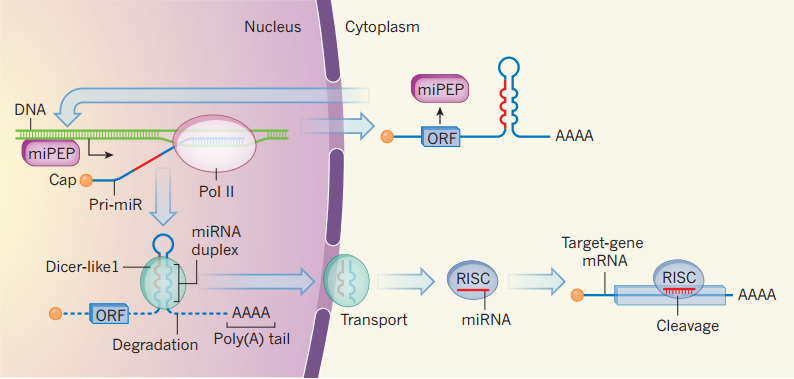
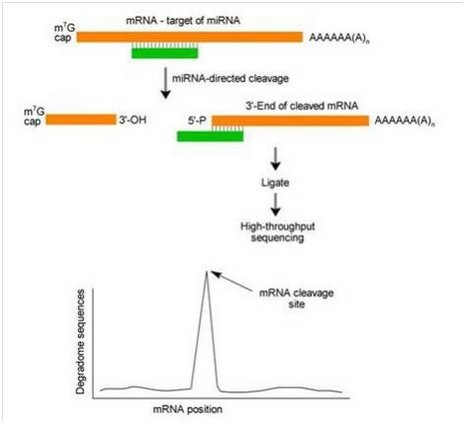
图片注释:MicroRNAs and their associated peptides. The precursors of plant microRNAs (miRNAs) are
pri-miR sequences, which are transcribed from DNA by the enzyme RNA polymerase II (Pol II). They are
then modified by capping and addition of a poly(A) tail. The miRNA duplexes are subsequently excised by
the enzyme Dicer-like1 and transported to the cytoplasm; other parts of the pri-miR are degraded. After
further processing, the resulting miRNA sequence guides repression of gene expression as part of the
RISC complex. Lauressergues et al.report that some pri-miRs contain short open reading frame (ORF)
sequences that can produce peptides (miPEP). The miPEPs enhance expression of the pri-miR, leading
to more miRNA and so more effective cleavage of the target gene’s messenger RNA. Such ORFs may avoid
degradation as part of pri-miRs that might exit the nucleus without being processed by Dicer-like1.

关键信息总结

1) Both plant and animal pri-miRs are transcribed from DNA in the nucleus by the enzyme RNA polymerase II.
2) The structured (fold-back) region of the transcript surrounding the miRNA sequence is recognized and processed by one of two enzymes-Drosha or Dicer-like1(In plants, Dicer-like1 cuts out the miRNA in a duplex form).
3) Transporter proteins export the excised sequences to the cytoplasm, where they are further processed before becoming competent to guide the RNA-induced silencing complex (RISC) in repressing target genes through either cleavage or translational repression of their mRNAs.
4) The miPEPs had the same tissue distribution as their associated mature miRNAs and enhanced the expression and effectiveness of these miRNAs. Moreover, the miPEPs promoted the transcription of their corresponding pri-miR, rather than enhancing miRNA stability.

miRNA合成途径

miRNA的合成大体经过:初级miRNA(pri-miRNA, primary miRNA)→前体miRNA(pre-miRNA, precursor-miRNA)→成熟miRNA(miRNA, mature miRNA)。
其具体合成途径存在两种形式:经典合成途径和Mirtron合成途径;
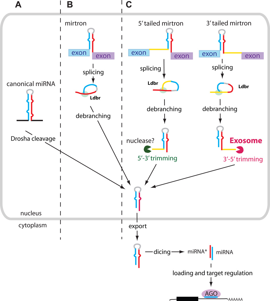
经典合成途径

来源:基因间隔区或编码基因内含子中;
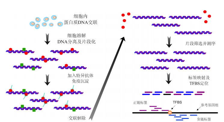
细胞核内编码miRNA 的基因通过RNA聚合酶II 或RNA聚合酶III 转录生成初级miRNA(pri-miRNA),pri-miRNA与来自蛋白质编码基因mRNA相似,有5’ 端帽式结构和3’ 端多聚腺苷酸尾结构,长度可达数千个碱基。接着pri-miRNA在一种RNaseIII(Drosha 酶)和它的伴侣分子(DiGeorge syndrome critical region gene 8,DGCR8)组成的复合物作用下,剪切为70~80 个核苷酸长度、具有茎环结构的miRNA 前体(pre-miRNA)。miRNA 前体在Ran-GTP 依赖的核质/ 细胞质转运蛋白——输出蛋白5(exportin 5)的作用下,从核内运输到胞质中。随后miRNA前体在另一种RNaseIII(Dicer酶)的作用下被剪切成21~25 个核苷酸长度,而且其5’端磷酸化和3’端有2 nt 的悬垂序列,类似于siRNA 的不完全配对的双链RNA,它们是由成熟miRNA与miRNA* 组成的二聚体,miRNA*是pre-miRNA中的一段RNA,其位置恰好与成熟的miRNA 相对。最后在RNA解旋酶作用下生成成熟miRNA 和miRNA*,成熟miRNA结合到RNA诱导的基因沉默复合物(RNA-induced silencing complex, RISC)中发挥作用,miRNA* 则被降解。
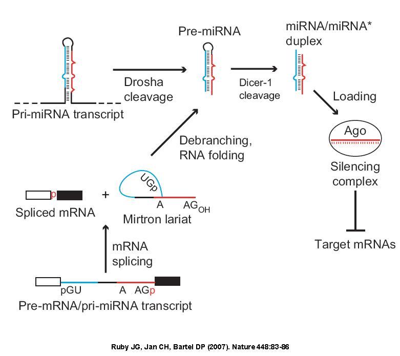
Mirtron途径

2007年,Ruby等在研究黑腹果蝇和秀丽隐杆线虫的小RNA 序列时首次发现mirtron,是一类定位于mRNA编码基因内含子内的miRNA,与经典miRNA合成相比其合成过程不需要经过Drosha酶切割,其形式功能与miRNA相同,具有以下特点:
(1)来自长度为56 nt 的内含子序列;
(2)能够形成miRNA:miRNA*复合物;
(3)内含子序列及其二级结构非常保守;
(4)内含子存在于基因组中的外显子中间并且有”GU-AG”的典型内含子特点;
(5)最后形成的成熟miRNA总来自于3’ 端侧的序列;
(6)合成需要Ldbr(lariat-debranching enzyme,套索分支酶)(参与内含子剪接) 的作用;
(7)与经典的miRNA一样,依赖Ran-GTP/ 输出蛋白5 的转运机制转运出核,在Dicer 酶的作用下成为成熟的miRNA。
同时,mirtron在哺乳动物中和在无脊椎动物中有明显的不同,如:
(1)哺乳动物中的mirtron途径合成的功能miRNA大多数来自mirtron的5’茎序列;
(2)不管哺乳动物中的mirtron3’ 茎序列能否成为成熟miRNA,它的起始核苷酸总是尿嘧啶(U)或胞嘧啶(C);
(3)哺乳动物中mirtron悬垂序列(overhang, 发夹结构末端突出序列)大多数为单核苷酸(G),只有少数是双核苷酸(AG);
(4)哺乳动物中mirtron比经典的miRNA前体和无脊椎动物mirtron的GC 含量要高,自由能要低。

阻断miRNA对mRNA的调控作用

miRNA海绵(miRNA sponges)

miRNA海绵是一种miRNA靶基因的竞争性抑制剂,是将若干个miRNA的反义序列串联在一起,连接到合适的载体中表达,其转录物”吸附”相应的miRNA,与miRNA靶基因形成竞争,导致靶基因去抑制化。
miRNA海绵表达载体的构建策略

circRNA

环状RNA(circRNA)对miRNA的吸附作用。http://tiramisutes.github.io/2016/04/12/Circular-RNAs/

miRNA数据库

miocroRNA databases:http://micrornadatabases.com/Databases.html

miRNA相关工具

mirtron prediction

Mirtron’SVM’prediction

MicroRNA Target Prediction

miRanda — miRNA target prediction for human, drosophila and zebrafish genomes
miRBase — a comprehensive repository for miRNAs and their predicted targets
miRDB — an online database for miRNA target prediction and functional annotations in animals
miRNAMap — a genomic maps of microRNA genes and their target genes in mammalian genomes
miR2Disease — a database providing comprehensive resource of miRNA deregulation in various human diseases
TarBase — a comprehensive database of experimentally supported animal microRNA targets
PicTar — microRNA targets for vertebrates, fly and nematodes
TargetScan — a search for the presence of conserved sites that match the seed of each miRNA
Target Gene Prediction at EMBL — miRNA-Target predictions for Drosophila miRNAs

Databases for microRNA Expression

microRNA.org — predicted microRNA targets & target downregulation scores. Experimentally observed expression patterns
HMDD — Human MicroRNA Disease Database (HMDD) is a database that contains the experimentally supported miRNA-disease
association data, which are manually curated from publications. The dysfunction evidence or miRNAs and literature PubMed ID are also given
TransmiR — a web query-driven database integrating the experimentally supported transcription factor and miRNA regulator relations

RNA Secondary Structure Prediction

DIANA MicroTest — a prediction of miRNA-mRNA interaction
mfold — tools for predicting the secondary structure of RNA and DNA, mainly by using thermodynamic methods
microInspector — a web tool for detection of miRNA binding sites in an RNA sequence
miRNA Bioinfor — miRNA End Energy calculator which takes miRNA duplex to calculate free energy for 5 base pairs at
one end plus a dangling nucleotide
miRRim — a method for detecting miRNA foldbacks based on hidden Markov model (HMM)
MXSCARNA — a multiple alignment tool for RNA sequences using progressive alignment based on pairwise structural alignment algorithm of SCARNA. Good for large scale analyses.
RNAhybrid— a tool for finding the minimum free energy hybridisation of a long and a short RNA

MicroRNA Homologous Prediction

miRNAminer — a web-based tool used for homologous miRNA gene search in several species
miRviewer — a global view of homologous miRNA genes in many species
RISCbinder— prediction of guide strand of microRNAs
Mireval — Sequence evaluation of microRNA properties

MicroRNA Deep Sequencing

miRanalyzer— A microRNA detection and analysis tool for next-generation sequencing experiments
miRNAkey— A software pipeline for the analysis of microRNA Deep Sequencing data
miRDeep— Discovering known and novel miRNAs from deep sequencing data

miRNA百科

microRNA.gene-quantification.info

参考文献:
Plant biology: Coding in non-coding RNAs
Mirtrons: microRNA biogenesis via splicing

ChIP-sequencing介绍

Posted on 2015-12-01 | In molecular biology | Comments: | Views: ℃
| Words count in article: | Reading time ≈

简介(From Wikipedia, the free encyclopedia)

ChIP-sequencing, also known as ChIP-seq, is a method used to analyze protein interactions with DNA. ChIP-seq combines chromatin immunoprecipitation (ChIP) with massively parallel DNA sequencing to identify the binding sites of DNA-associated proteins. It can be used to map global binding sites precisely for any protein of interest. Previously, ChIP-on-chip was the most common technique utilized to study these protein–DNA relations.
ChIP-seq is used primarily to determine how transcription factors and other chromatin-associated proteins influence phenotype-affecting mechanisms. Determining how proteins interact with DNA to regulate gene expression is essential for fully understanding many biological processes and disease states.

流程

ChIP

The ChIP process enriches specific crosslinked DNA-protein complexes using an antibody against the protein of interest. For a good description of the ChIP wet lab protocol see ChIP-on-chip. Oligonucleotide adaptors are then added to the small stretches of DNA that were bound to the protein of interest to enable massively parallel sequencing.

Sequencing

After size selection, all the resulting ChIP-DNA fragments are sequenced simultaneously using a genome sequencer. A single sequencing run can scan for genome-wide associations with high resolution, as opposed to large sets of tilingarrays required for lower resolution ChIP-chip.

中文解释


ChIP 测序的基本原分为 ChIP 和测序两个步骤。ChIP 是英文 Chromatin immunoprecipitation 的缩写,即染色质免疫沉淀,其步骤包括:细胞内蛋白质和 DNA 的交联、DNA 分子分离及片段化、免疫沉淀和解除交联。测序就是对解除交联后的 DNA 片段进行测序,制备文库时也包括连接测序接头和片段筛选等步骤。由于免疫沉淀的 DNA 片段在蛋白质结合区域周围富集,因此识别蛋白质结合区域转化为检测测序标签富集的区域。在信息处理中,这是一个信号检测的问题。在转录因子 ChIP 测序数据分析中,由于测序标签还会在转录因子结合位点周围形成分布,通过对分布的统计建模分析,可从数据中精确定位结合位点。

Computational analysis

The read count data generated by ChIP-seq is massive. It motivates the development of computational analysis methods. To predict DNA-binding sites from ChIP-seq read count data, peak calling methods have been developed. The most popular method is MACS which empirically models the shift size of ChIP-Seq tags, and uses it to improve the spatial resolution of predicted binding sites.[10]

Another relevant computational problem is Differential peak calling, which identifies significant differences in two ChIP-seq signals from distinct biological conditions. Differential peak callers segment two ChIP-seq signals and identify differential peaks using Hidden Markov Models. Examples for two-stage differential peak callers are ChIPDiff[11] and ODIN.
具体数据分析详细见:http://www.plob.org/2012/09/29/3760.html

Contribution from :
https://en.wikipedia.org/wiki/ChIP-sequencing
http://www.illumina.com/documents/products/datasheets/datasheet_chip_sequence.pdf
http://bioinfo.au.tsinghua.edu.cn/member/xwang/files/Thesis_XiWang_OL.pdf

Linux 下批量下载 http 中链接内容

Posted on 2015-12-01 | In Linux | Comments: | Views: ℃
| Words count in article: | Reading time ≈


KOBAS这个软件所需数据库有3540个物种数据,如何实现批量下载…

察看html网页源文件可发现:所有这些下载链接都整齐排列于 KO
这样一个html语法结构中,所以可以通过正则表达式匹配找出所有的下载链接;

方法1:python抓取网页并下载

python中实现爬虫,解析网页html文件和下载文件的简单容易上手的优秀模块分别为requests,BeautifulSoup和re,通过三者的组合可实现爬虫网页并批量下载。
导入所需模块

1
2
3
4
5
6
7
8
9
10
11
12
13
14
15
16
17
18
19
20
21
22
23
24
25
26
27
28
29
30
31
32
#!~/bin/Python-2.7.10/
from BeautifulSoup import BeautifulSoup
import requests
import re
#—--name:url-batch-download.py--
#—--修改:hope--
# point to output directory
outpath = '/backend3/'
url = 'http://kobas.cbi.pku.edu.cn/site/download_db.jsp'
mbyte=1024*1024

print 'Reading: ', url
html = requests.get(url).text
soup = BeautifulSoup(html)

print 'Processing: ', url
for name in soup.findAll('a', href=True):
gzurl = name['href']
strinfo = re.compile('\../')
xzp= strinfo.sub('http://kobas.cbi.pku.edu.cn/',gzurl)
print xzp
if( xzp.endswith('.gz') ):
outfname = outpath + xzp.split('/')[-1]
r = requests.get(xzp, stream=True)
if( r.status_code == requests.codes.ok ) :
fsize = int(r.headers['content-length'])
print 'Downloading %s (%sMb)' % ( outfname, fsize/mbyte )
with open(outfname, 'wb') as fd:
for chunk in r.iter_content(chunk_size=1024): # chuck size can be larger
if chunk: # ignore keep-alive requests
fd.write(chunk)
fd.close()

修稿py文件为可执行文件

1
chmod +x url-batch-download.py

开始爬虫并批量下载

1
python2.7 url-batch-download.py

方法2:wget批量下载
1) wget下载整个html页面后批量下载
wget都很熟悉,但是通常只是用来下载单个文件,如果需要批量下载呢?

1
wget http://kobas.cbi.pku.edu.cn/site/download_db.jsp

对于这个链接下载完后是jsp后缀文件,可以重命名为index.html。
2) 开始批量下载

1
wget -i index.html -F -B http://kobas.cbi.pku.edu.cn/site/download_db.jsp

参数解释:
-i 表示从文件导入链接,默认是直接按行读取URL
-F 表示将文件以HTML的格式解析,其实就是解析
-B 因为发现解析出来的链接用的都是相对路径,而为了下载这个文件,必须在相对路径前添加上Base URL,-B就是用来添加Base URL。

这样就可以批量下载当前目录中的文件了。

DNA methylation

Posted on 2015-11-30 | In molecular biology | Comments: | Views: ℃
| Words count in article: | Reading time ≈

简介

DNA methylation is a process by which methyl groups are added to DNA. Methylation modifies the function of the DNA. When located in a gene promoter, DNA methylation typically acts to repress gene transcription. DNA methylation is essential for normal development and is associated with a number of key processes including genomic imprinting, X-chromosome inactivation, repression of repetitive elements, and carcinogenesis.
DNA methylation at the 5 position of cytosine has the specific effect of reducing gene expression and has been found in every vertebrate examined. In adult somatic cells (cells in the body, not used for reproduction), DNA methylation typically occurs in a CpG dinucleotide context; non-CpG methylation is prevalent in embryonic stem cells,[5][6][7] and has also been indicated in neural development.

原理

在甲基转移酶的催化下,DNA的CG两个核苷酸的胞嘧啶被选择性地添加甲基,形成5-甲基胞嘧啶,这常见于基因的5’-CG-3’序列。大多数脊椎动物基因组DNA都有少量的甲基化胞嘧啶,主要集中在基因5’端的非编码区,并成簇存在。甲基化位点可随DNA的复制而遗传,因为DNA复制后,甲基化酶可将新合成的未甲基化的位点进行甲基化。DNA的甲基化可引起基因的失活,DNA甲基化导致某些区域DNA构象变化,从而影响了蛋白质与DNA的相互作用,甲基化达到一定程度时会发生从常规的B-DNA向Z-DNA的过渡,由于Z-DNA结构收缩,螺旋加深,使许多蛋白质因子赖以结合的原件缩入大沟而不利于转录的起始,导致基因失活。
DNA甲基化主要形成5-甲基胞嘧啶(5-mC)和少量的N6-甲基腺嘌呤(N6-mA)及7-甲基鸟嘌呤(7-mG)。

结构基因编辑

含有很多CpG 结构,2CpG 和2GPC 中两个胞嘧啶的5 位碳原子通常被甲基化,且两个甲基集团在DNA 双链大沟中呈特定三维结构。基因组中60%~ 90% 的CpG 都被甲基化,未甲基化的CpG 成簇地组成CpG 岛,位于结构基因启动子的核心序列和转录起始点。有实验证明超甲基化阻遏转录的进行。DNA 甲基化可引起基因组中相应区域染色质结构变化,使DNA 失去核酶ö限制性内切酶的切割位点,以及DNA 酶的敏感位点,使染色质高度螺旋化,凝缩成团,失去转录活性。5 位C 甲基化的胞嘧啶脱氨基生成胸腺嘧啶,由此可能导致基因置换突变,发生碱基错配: T2G,如果在细胞分裂过程中不被纠正,就会诱发遗传病或癌症,而且,生物体甲基化的方式是稳定的,可遗传的。

The Role of Methylation in Gene Expression

1) Not all genes are active at all times. DNA methylation is one of several epigenetic mechanisms that cells use to control gene expression.
2) 5-azacytidine Experiments Provide Early Clues to the Role of Methylation in Gene Expression.

候选基因CpG岛区域和候选基因甲基化与表观基因组学


1
2
3
4
5
6
7
Figure 1 | Altered DNA-methylation patterns in tumorigenesis. The hypermethylation of CpG islands of tumoursuppressor
genes is a common alteration in cancer cells, and leads to the transcriptional inactivation of these genes
and the loss of their normal cellular functions. This contributes to many of the hallmarks of cancer cells. At the same
time, the genome of the cancer cell undergoes global hypomethylation at repetitive sequences, and tissue-specific
and imprinted genes can also show loss of DNA methylation. In some cases, this hypomethylation is known to
contribute to cancer cell phenotypes, causing changes such as loss of imprinting, and might also contribute to the
genomic instability that characterizes tumours. E, exon.

如图1左所示,在正常细胞中,位于抑癌基因启动子区域的CpG岛处于低水平或未甲基化状态,此时抑癌基因处于正常的开放状态,抑癌基因不断表达抑制肿瘤的发生。而在肿瘤细胞中,该区域的CpG岛被高度甲基化,染色质构象发生改变,抑癌基因的表达被关闭,从而导致细胞进入细胞周期,凋亡丧失,DNA修复缺陷,血管生成以及细胞粘附功能缺失等,最终导致肿瘤发生。同样,如图1右所示,对于在正常细胞中处于高度甲基化的一些基因和重复序列,如果其甲基化水平降低,这些基因将表达和重复序列将激活,从而导致基因印记丢失,细胞过度增长,不合适的细胞特异性表达,基因组脆性增加,以及内寄生序列(endoparasitic sequence)的激活,最终也导致肿瘤发生。

DNA甲基化检测方法

据检测样本不同,可以分为DNA和mRNA。现有方法,绝大部分都是取样于细胞的DNA,根据研究水平,又将这些方法归为3大类,即:基因组甲基化水平(Methylation Content)的分析,候选基因甲基化分析,和基因组层次的DNA甲基化模式(Methylation pattern)与甲基化谱(Methylation Profiling)分析。

基因组甲基化水平(Methylation Content)

高效液相色谱(High-performance Liquid Chromatography, HPLC)

根据DNA或蛋白分子量和构象的不同而使其加以分离。由于在动态相和静态相下分子的光吸收度并不相同而加以定量。随着系统的压强的增加,其分辨率增高。故而能够定量测定基因组整体水平DNA甲基化水平。
过程是将DNA样品先经盐酸或氢氟酸水解成碱基,水解产物通过色谱柱,结果与标准品比较,用紫外光测定吸收峰值及其量,计算5 mC/(5mC+5C)的积分面积就得到基因组整体的甲基化水平。这是一种检测DNA甲基化水平的标准方法。

高效毛细管电泳法(High-performance Capillary Electrophoresis, HPCE)

利用窄孔熔融石英毛细管来从复合物中分离不同化学组分的技术。其基础是在强电场下不同分子的由于其所带电荷,大小,结构以及疏水性等不同而相互分开。用HPCE方法处理DNA水解产物来确定5mC水平,简便,经济且敏感性高。
以上各种方法虽然能够明确检测出目的序列中所有CpG位点的甲基化状况,但并不能对甲基化位点进行定位。

候选基因(Candidate Gene)

甲基化敏感性限制性内切酶-PCR/Southern法( methylation-sensitive restriction Endonuclease -PCR/Southern, MSRE-PCR/Southern)

这种方法利用甲基化敏感性限制性内切酶对甲基化区的不切割的特性,将DNA消化为不同大小的片段后,进行Southern或PCR扩增分离产物,明确甲基化状态再进行分析。常使用的甲基化敏感的限制性内切酶有HpaⅡ-MspⅠ(CCGG)和SmaⅠ-Xmal(CCCGGG)等。

重亚硫酸盐测序法(Bisulphite Sequencing)

该方法首先用重亚硫酸盐使DNA中未发生甲基化的胞嘧啶脱氨基转变成尿嘧啶,而甲基化的胞嘧啶保持不变,行PCR扩增所需片段,则尿嘧啶全部转化成胸腺嘧啶,最后,对PCR产物进行测序并且与未经处理的序列比较,判断是否CpG位点发生甲基化。此方法是精确度很高,能明确目的片段中每一个CpG位点的甲基化状态,但需要大量的克隆测序,过程较为繁琐、昂贵。

甲基化特异性的PCR(methylation-specific PCR, MS-PCR)

该方法同样DNA先用重亚硫酸盐处理,随后行引物特异性的PCR。其设计两对引物,分别与重亚硫酸盐处理后的序列互补配对,即一对结合处理后的甲基化DNA链,另一对结合处理后的非甲基化DNA链。检测MS-PCR扩增产物,如果用针对处理后甲基化DNA链的引物能扩增出片段,则说明该被检测的位点存在甲基化;反之亦然。

甲基化荧光法(MethyLight)

结合重亚硫酸盐处理待测DNA片段,设计一个能与待测位点区互补的探针,探针的5’端连接报告荧光,3’端连接淬灭荧光,随后行实时定量PCR。如果探针能够与DNA杂交,则在PCR用引物延伸时,TaqDNA聚合酶5′到3′端的外切酶活性会将探针序列上5′端的报告荧光切下,淬灭荧光不再能对报告荧光进行抑制,这样报告荧光发光,测定每个循环报告荧光的强度即可得到该位点的甲基化情况及水平。本方法高效,迅速,具备可重复、所需样本量少、不需要电泳分离的特点。

焦磷酸测序(Pyrosequencing)

该方法,由4种酶催化同一反应体系中的酶级联化学发光反应,在每一轮测序反应中,只加入一种dNTP,若该dNTP与模板配对,聚合酶就能将其加入到引物链中并释放出等摩尔数的焦磷酸(PPi)。PPi可最终转化为可见光信号,并由PyrogramTM转化为一个峰值,其高度与核苷酸数目成正比。当用于甲基化检测时,经重亚硫酸盐处理的序列可以看作是C-T型的SNP改变。其操作简单,结果准确可靠,可以行大规模分析。

结合重亚硫酸盐的限制性内切酶法(combined bisulfiterestriction analysis, COBRA)

这种方法对标本DNA行重亚硫酸盐处理及PCR扩增,处理后原甲基化的胞嘧啶被保留,而非甲基化的胞嘧啶变为胸腺嘧啶。随后用限制性内切酶对转化后PCR产物切割的特性以识别原标本DNA的甲基化状况。该方法相对简单,不需预先知道CpG位点及样本序列。

基因组范围的DNA甲基化模式(Methylation pattern)与甲基化谱(Methylation Profiling)

限制性标记基因组扫描(Restriction Landmark Genomic Scanning, RLGS)

RLGS是最早适用于基因组范围DNA甲基化分析的方法之一。该方法先用甲基化敏感的稀频限制性内切酶NotⅠ消化基因组DNA,甲基化位点保留,标记末端、切割、行一维电泳,随后再用更高频的甲基化不敏感的内切酶切割,行二维电泳,这样甲基化的部分被切割开并在电泳时显带,得到RLGS图谱与正常对照得出缺失条带即为甲基化的可能部位。

甲基化间区位点扩增(amplification of inter-methylated sites, AIMS)

AIMS是基于任意引物PCR(Arbitrary Primed PCR)的一种方法,由于任意引物PCR使用寡核苷酸连接子(linker) 进行连接,不需要依赖任何序列的先验信息。在该方法中,用来进行扩增的模板序列首先通过甲基化敏感的限制性内切酶进行消化而富集,其特异性由该酶酶切片断一端的特定序列结合连接子来保证。随后,由内切酶进行第二次消化,再次连接,提纯进行PCR扩增,最后电泳,提取目的序列进行测序。

甲基化CpG岛扩增(Methylated CpG-island amplification, MCA)

MCA也是基于任意引物PCR的方法,该方法使用两种对甲基化具有不同敏感度的限制性内切酶(如SmaI和XmaI)先后进行消化,然后对甲基化敏感的限制性酶切片断进行接头(Adaptor)连接,行PCR,那些富含CpG的序列就会被选择性的扩增。该方法对甲基化分析和克隆甲基化差异性基因都非常有帮助。

差异甲基化杂交(Differential Methylation Hybridization,DMH)

DMH属于一种芯片技术,在该技术中,包括扩增子(Amplicon)生成和CGI文库筛选两个重要组成部分。在扩增子生成中,首先用MseI来酶切DNA样本,然后接上连接子,并去除重复序列,这时的样本一分为二,其一直接进行PCR扩增,生成仅由MseI处理过的扩增子,而另一半则用甲基化敏感的酶BstUI进行消化,然后进行PCR扩增,生成由MseI/BstUI共同处理过的扩增子。CGI文库通过筛查出重复序列,然后进行PCR,选出含有BstUI位点的克隆,最后这些克隆一式两份点到芯片上,制备成CGI芯片。然后把两种不同的扩增子分别杂交到相应的CGI克隆点上,最后通过差异性对比检测出那些未甲基化位点。

由连接子介导PCR出的HpaII小片断富集分析(HpaII tiny fragement Enrichment by Ligation-mediated PCR, HELP)

该方法用HpaII与其对甲基化敏感同裂酶MspI对同一基因组序列进行消化,产生不同的代表性序列,然后对此序列进行连接子介导的PCR,瑞和进行电泳等比较分析或将此DNA样本共杂交到基因组芯片上进行分析。这种方法已经揭示了大量的组织特异性,差异甲基化区域,并用于正常细胞和癌症细胞的基因组比较分析。

甲基化DNA免疫沉淀法(Methylated DNA immunoprecipitation, MeDIP)

这是一种高效富集甲基化DNA的方法。在该方法中,可与5mC特异性结合的抗体加入到变性的基因组DNA片段中,从而使甲基化的基因组片断免疫沉淀,形成富集。通过与已有DNA微芯片技术相结合,从而进行大规模DNA甲基化分析。该方法简便,特异性高,适合DNA甲基化组学(DNA Methylome)的分析。

候选基因甲基化分析网址

http://katahdin.mssm.edu/kismeth/revpage.pl
Contribution from :http://www.nature.com/scitable/topicpage/the-role-of-methylation-in-gene-expression-1070
http://www.nature.com/nrg/journal/v8/n4/full/nrg2005.html
http://www.lifeomics.com/?p=18458

甲基化引物设计

Methyl Primer Express® Software v1.0
https://www.thermofisher.com/order/catalog/product/4376041

Degradome-降解组

Posted on 2015-11-30 | In Bioinformatics | Comments: | Views: ℃
| Words count in article: | Reading time ≈

Degradome sequencing

Degradome sequencing (Degradome-Seq),also referred to as parallel analysis of RNA ends (PARE),is a modified version of 5’-Rapid Amplification of cDNA Ends (RACE) using high-throughput, deep sequencing method using as Illumina’s SBS technology. Degradome sequencing provides a comprehensive means of analyzing patterns of RNA degradation.

Degradome sequencing has been used to identify microRNA (miRNA) cleavage sites,because miRNAs can cause endonucleolytic cleavage of mRNA by extensive and often perfect complementarity to mRNAs.Degradome sequencing revealed many known and novel plant miRNA (siRNA) targets. Recently, degradome sequencing also has been applied to identify animal (human and mouse) miRNA-derived cleavages.

原理


在植物体内绝大多数的miRNA是利用剪切作用调控靶基因的表达,且剪切常发生在miRNA与mRNA互补区域的第十位核苷酸上。靶基因经剪切产生二个片段,5’ 剪切片段和3’ 剪切片段。其中3’ 剪切片段,包含有自由的5’ 单磷酸和3’ polyA尾巴,可被RNA连接酶连接,连接产物可用于下游高通量测序;而含有5’ 帽子结构的完整基因,含有帽子结构的5’ 剪切片段或是其他缺少5’ 单磷酸基团的RNA是无法被RNA酶连接的,因而无法进入下游的测序实验;对测序数据进行深入地比对分析,可以直观地发现在mRNA序列的某个位点会出现一个波峰,而该处正是候选的miRNA剪切位点。

測序數據的分析方法

測序數據使用賓州大學 Addo-Quaye 等建立CleaveLand 分析方法進行比對分析,可以直觀地發現在 mRNA 序列的某個位點會出現一個波峰,而該處正是候選的 miRNA 剪切位元點。

Fluorescence in situ Hybridization(荧光原位杂交)

Posted on 2015-11-29 | In molecular biology | Comments: | Views: ℃
| Words count in article: | Reading time ≈

简介

荧光原位杂交(fluorescence in situ hybridization,FISH)是在20世纪80年代末在放射性原位杂交技术的基础上发展起来的一种非放射性分子细胞遗传技术,以荧光标记取代同位素标记而形成的一种新的原位杂交方法。探针首先与某种介导分子(reporter molecule)结合,杂交后再通过免疫细胞化学过程连接上荧光染料。FISH的基本原理是将DNA(或RNA)探针用特殊的核苷酸分子标记,然后将探针直接杂交到染色体或DNA纤维切片上,再用与荧光素分子偶联的单克隆抗体与探针分子特异性结合来检测DNA序列在染色体或DNA纤维切片上的定性、定位、相对定量分析。FISH具有安全、快速、灵敏度高、探针能长期保存、能同时显示多种颜色等优点,不但能显示中期分裂相,还能显示于间期核。同时在荧光原位杂交基础上又发展了多彩色荧光原位杂交技术和染色质纤维荧光原位杂交技术.。

Preparation and hybridization process – DNA


First, a probe is constructed. The probe must be large enough to hybridize specifically with its target but not so large as to impede the hybridization process. The probe is tagged directly with fluorophores, with targets for antibodies or with biotin. Tagging can be done in various ways, such as nick translation, or PCR using tagged nucleotides.

Then, an interphase or metaphase chromosome preparation is produced. The chromosomes are firmly attached to a substrate, usually glass. Repetitive DNA sequences must be blocked by adding short fragments of DNA to the sample. The probe is then applied to the chromosome DNA and incubated for approximately 12 hours while hybridizing. Several wash steps remove all unhybridized or partially hybridized probes. The results are then visualized and quantified using a microscope that is capable of exciting the dye and recording images.

If the fluorescent signal is weak, amplification of the signal may be necessary in order to exceed the detection threshold of the microscope. Fluorescent signal strength depends on many factors such as probe labeling efficiency, the type of probe, and the type of dye. Fluorescently tagged antibodies or streptavidin are bound to the dye molecule. These secondary components are selected so that they have a strong signal.

Difference between Southern Blot and Fluorescence in situ hybridization (FISH) ?

FISH is performed on intact chromosomes through interphase or metaphase.it doesnt need DNA extraction and is performed on microscopic slides. its a type of kariotyping.its use is to determine the chromosomal abberations(numerical and structural) of a patient.
But,in Southern blotting you should first extract DNA of the specimen then cleave it with a restriction enzyme and then run on gel electrophoresis. the next step is to blot the DNA on a membrane and hybridaze it with a labeled probe. the use of suthern blot is in detecting mutations and restriction length fragment polymorphysms.
https://answers.yahoo.com/question/index?qid=20120611095540AA1YXhl

R数据整形术之plyr

Posted on 2015-11-29 | In R | Comments: | Views: ℃
| Words count in article: | Reading time ≈

plyr包可以进行类似于数据透视表的操作,将数据分割成更小的数据,对分割后的数据进行些操作,最后把操作的结果汇总。
本文主要介绍以下内容:
Split-Aapply-Combine 原理介绍
baby_names的名字排名
求分段拟合的系数
部分其他函数介绍
在正式开始之前,请确保电脑上已经安装plyr,如果没有,通过install.packages()函数安装。

1
2
3
4
5
6
7
8
9
10
11
> require(plyr)  #载入plyr包
> ##假设有美国新生婴儿的取名汇总,每一年,会统计男孩和女孩的取名情况,形成如下的一张表。baby_names数据集包含1880 ~ 2008年间的数据, 包含统计的年份(year),新生婴儿的性别、名字、以及改名字的比例。
> baby_names<-read.csv("baby-names.csv")
> head(baby_names)
year name percent sex
1 1880 John 0.081541 boy
2 1880 William 0.080511 boy
3 1880 James 0.050057 boy
4 1880 Charles 0.045167 boy
5 1880 George 0.043292 boy
6 1880 Frank 0.027380 boy

以提问并解决问题的形式对plyr做介绍。

想知道数据集中,每年都有多少记录?
数据集中,男孩和女孩名的各自排名?
男孩名和女孩名各自排名前100在当年中的比例?
数据集中,每年都有多少记录
先假设我们有某一年的数据,我们会如何统计其中的记录数呢?由于数据集中,每条记录一行,只需要统计对应的行数就可以得到对应的记录数。
写个函数试试

1
2
3
> record_count <- function(df) {
+ return(data.frame(count = nrow(df)))
+ }

返回值类型是data.frame类型,是为即将介绍的ddply()函数做铺垫。先来看看2008年,数据集中有多少记录。

1
2
3
4
> baby_names_2008 <- subset(baby_names, year == 2008)
> record_count(baby_names_2008)
count
1 2000

结果显示2000条,貌似我们已经得到答案。下面想想,该如何得到1880 ~ 2008这129年间,每年的记录数呢?

1
2
3
4
5
6
7
8
9
10
11
12
13
14
> baby_names_1880_2008<-ddply(baby_names,     # 数据集
+ .(year), # 分类的标准
+ record_count # 函数
+ )
> head(baby_names_1880_2008)
year count
1 1880 2000
2 1881 2000
3 1882 2000
4 1883 2000
5 1884 2000
6 1885 2000
> dim(baby_names_1880_2008)
[1] 129 2

ddply解释:
定义了一个负责计数的函数record_count()
调用ddply(),这里出现刚刚定义的函数
ddply()函数是plyr包中用于对data.frame结构的数据做处理的函数,其结果也是data.frame。ddply的参数列表如下:

1
2
ddply(.data, .variables, .fun = NULL, ..., .progress = "none",
.inform = FALSE, .drop = TRUE, .parallel = FALSE, .paropts = NULL)

各部分解释如下
第一个参数是要操作的原始数据集,比如babyname
第二个参数是按照某个(也可以几个)变量,对数据集分割,比如按照year对数据集分割,可以写成.(year)的形式
第三个参数是具体执行操作的函数,对分割后的每一个子数据集,调用该函数
第四个参数可选,表示第三个参数对应函数所需的额外参数
其他参数,可以暂时不用考虑。ddply()函数会自动的将分割后的每一小部分的计算结果汇总,以data.frame的格式保存。分割后的数据,是fun的第一个参数。
在上面的描述中,提到的分割、_操作、汇总
,在plyr包中是一种处理方式(“frame”),即”Split - Apply - Combine”。在plyr包中有很多这种处理方式的函数,在介绍这些函数之前,我们再来看看ddply()的一些更深入的用法。

各年,男孩名与女孩名的各自排名

以2008年的数据为例,男孩名”Jacob”的比例最高,排名应当是第一,”Michael”紧跟其后,排名应当第二,依此类推。对于女孩名,”Emma”排名第一,”Isabella”排名第二,”Emily”排名第三等等。我们希望得到这样的结果。

对于2008年的数据,可以通过简单的rank即可得到,不过要对男孩和女孩分别排序。

1
2
3
baby_names_2008_boy <- subset(baby_names_2008, sex == "boy") # 获取男孩名
baby_names_2008_boy$rank <- rank(- baby_names_2008_boy$percent) # 排序
head(baby_names_2008_boy) # 查看

如何利用ddply()对原始数据集做相应的操作呢?这里需要介绍R语言中的一个函数transform(),该函数对原始数据集做一些操作,并把结果存储在原始数据中,更详细的用法,参见帮助文档?transform。

第一个版本的处理方式是这样的

1
2
3
4
5
ddply(baby_names, 
.(year, sex),
transform,
rank = rank(-percent, ties.method = "first")
)

第二个参数有点变化,除了year,还有sex,这表示对baby_name数据集,对year和sex分类(类似于SQL中的group by year, sex)。
第四个参数是transform的额外参数,如果查看transform的帮助文档,其函数调用方式如下:

1
transform(_data, ...)

第一参数为操作的数据,在ddply()中为按年份和性别分割后的子数据集;后面的…参数是tag = value的形式,这种tag:value将追加在数据中。
由于rank默认对数据进行升序排序,若要实现逆序排序,常规的做法是将数据的符号取反,这也就是上面的rank函数中出现-percent的原因。在plyr中,有一个类似的函数,实现取反的操作,是desc。

1
2
3
x <- 1:10
desc(x)
# -1 -2 -3 -4 -5 -6 -7 -8 -9 -10

所以,上面对percent取反的操作,可以写得更优雅些,就有了第二个版本的函数

1
2
3
4
5
baby_names <- ddply(baby_names, 
.(year, sex),
transform,
rank = rank(desc(percent), ties.method = "first")
)

注意这里把结果赋给了baby_name,因为后面还会用到排名的信息,就把结果保存下来。

排名前100的男孩名与女孩名在当年中的比例

跟前一问类似,处理方法是:

把每年排名前100的数据筛选出来
把男孩和女孩对应的percent相加

1
2
3
4
5
baby_names_top100 <- subset(baby_names, rank <= 100)  # 将前100排名的数据筛选出来
baby_names_top100_trend <- ddply(baby_names_top100,
.(year, sex), # 按年和性别分割
summarize, # 汇总数据
trend = sum(percent)) # 汇总方式(求和)

这里出现一个新的操作函数summarize(),该函数是对数据做汇总,与transform不一样的是,该函数并不追加结果到原始数据,而是产生新的数据集。比如想知道,2008年的男孩名中,排名最高和最低的名字的百分比之差,可以通过如下方式求得:

1
2
summarize(baby_names_2008_boy, trend = max(percent) - min(percent))
# 0.010266

回到刚才的问题,从1880 ~ 2008年间,男孩名与女孩名的前100所占比例(可以衡量名字大众化的程度)到底是什么样的呢?画个图就知道了。

Contribution from :http://www.jianshu.com/p/bfddfe29aa39

R数据整形术之reshape2

Posted on 2015-11-29 | In R | Comments: | Views: ℃
| Words count in article: | Reading time ≈

数据类型

宽数据

1
2
3
4
5
#   ozone   wind  temp
# 1 23.62 11.623 65.55
# 2 29.44 10.267 79.10
# 3 59.12 8.942 83.90
# 4 59.96 8.794 83.97

长数据

1
2
3
4
5
6
7
8
9
10
11
12
13
#    variable  value
# 1 ozone 23.615
# 2 ozone 29.444
# 3 ozone 59.115
# 4 ozone 59.962
# 5 wind 11.623
# 6 wind 10.267
# 7 wind 8.942
# 8 wind 8.794
# 9 temp 65.548
# 10 temp 79.100
# 11 temp 83.903
# 12 temp 83.968

长数据有一列数据是变量的类型,有一列是变量的值。长数据不一定只有两列。ggplot2需要长类型的数据,plyr也需要长类型的数据,大多数的模型(比如lm(), glm()以及gam())也需要长数据。

reshape2 包

reshape2 用得比较多的是melt和cast两个函数。

melt函数对宽数据进行处理,得到长数据;
cast函数对长数据进行处理,得到宽数据;

melt函数

melt(参数)

1
2
3
melt(data,id.vars,measure.vars,
variable.name = "variable", ..., na.rm = FALSE,
value.name = "value")

其中id.vars可以指定一系列变量,然后measure.vars就可以留空了,这样生成的新数据会保留id.vars的所有列,然后增加两个新列:variable和value,一个存储变量的名称一个存储变量值。
此处用R内置的airquality数据集

1
2
3
4
5
6
7
8
> head(airquality)
Ozone Solar.R Wind Temp Month Day
1 41 190 7.4 67 5 1
2 36 118 8.0 72 5 2
3 12 149 12.6 74 5 3
4 18 313 11.5 62 5 4
5 NA NA 14.3 56 5 5
6 28 NA 14.9 66 5 6

首先将列名改成小写,然后查看相应的数据

1
2
3
4
5
6
7
8
9
10
11
12
13
14
15
16
17
18
19
20
21
22
23
24
25
26
27
28
29
> names(airquality)<- tolower(names(airquality))
> head(airquality)
ozone solar.r wind temp month day
1 41 190 7.4 67 5 1
2 36 118 8.0 72 5 2
3 12 149 12.6 74 5 3
4 18 313 11.5 62 5 4
5 NA NA 14.3 56 5 5
6 28 NA 14.9 66 5 6
##直接用metl函数处理上述的数据
> library("reshape2")
> aql <- melt(airquality)
No id variables; using all as measure variables
> head(aql)
variable value
1 ozone 41
2 ozone 36
3 ozone 12
4 ozone 18
5 ozone NA
6 ozone 28
> tail(aql)
variable value
913 day 25
914 day 26
915 day 27
916 day 28
917 day 29
918 day 30

默认情况下,melt认为所有数值列的变量均有值。很多情况下,这都是我们想要的情况。在这里,我们想知道每个月(month)以及每天(day)的ozone, solar.r, wind以及temp的值。因此,我们需要告诉melt,month和day是”ID variables”。ID variables就是那些能够区分不同行数据的变量,个人感觉类似于数据库中的主键。

1
2
3
4
5
6
7
8
9
> aql <- melt(airquality, id.vars = c("month", "day"))
> head(aql)
month day variable value
1 5 1 ozone 41
2 5 2 ozone 36
3 5 3 ozone 12
4 5 4 ozone 18
5 5 5 ozone NA
6 5 6 ozone 28

如果我们想修改长数据中的列名,该如何操作呢?

1
2
3
4
5
6
7
8
9
10
11
> aql <- melt(airquality, id.vars = c("month", "day"),
+ variable.name = "climate_variable",
+ value.name = "climate_value")
> head(aql)
month day climate_variable climate_value
1 5 1 ozone 41
2 5 2 ozone 36
3 5 3 ozone 12
4 5 4 ozone 18
5 5 5 ozone NA
6 5 6 ozone 28

cast函数

从宽格式数据变换到长格式的数据比较直观,然后反过来则需要一些二外的功夫。

在reshape2中有好几个cast版本的函数。若你经常使用data.frame,就需要使用dcast函数。acast函数返回向量、矩阵或者数组。

dcast借助于公式来描述数据的形状,左边参数表示”ID variables”,而右边的参数表示measured variables。可能需要几次尝试,才能找到合适的公式。

这里,我们需要告知dcast,month和day是ID variables,variable则表示measured variables。

1
2
3
4
5
6
7
8
9
10
11
12
13
14
15
16
17
18
> aql <- melt(airquality, id.vars = c("month", "day"))
> aqw <- dcast(aql, month + day ~ variable)
> head(aqw)
month day ozone solar.r wind temp
1 5 1 41 190 7.4 67
2 5 2 36 118 8.0 72
3 5 3 12 149 12.6 74
4 5 4 18 313 11.5 62
5 5 5 NA NA 14.3 56
6 5 6 28 NA 14.9 66
> head(airquality) # 与原始数据比较
ozone solar.r wind temp month day
1 41 190 7.4 67 5 1
2 36 118 8.0 72 5 2
3 12 149 12.6 74 5 3
4 18 313 11.5 62 5 4
5 NA NA 14.3 56 5 5
6 28 NA 14.9 66 5 6

If it isn’t clear to you what just happened there, then have a look at this illustration:

蓝色阴影块是能够表示每一行数据的ID variables;红色阴影块包含了将待生成数据的列名;而灰色的数据表示用于填充相关区域的数据。
令人产生疑惑的情况往往是,一个数据单元有一个以上的数据。比如,我们的ID variables不包含day,

1
2
3
4
5
6
7
8
> dcast(aql, month ~ variable)
Aggregation function missing: defaulting to length
month ozone solar.r wind temp
1 5 31 31 31 31
2 6 30 30 30 30
3 7 31 31 31 31
4 8 31 31 31 31
5 9 30 30 30 30

再次查看dcast的输出数据,可以看到每个单元是month与climate组合的个数。所得到数据是month对应的day的记录数。当每个单元有多个数据是,需要告诉dcast如何聚合(aggregate)这些数据,比如取均值(mean),计算中位数(median),或者简单的求和(sum)。比如,在这里,我们简单的计算下均值,同时通过na.rm = TRUE删除NA值。

1
2
3
4
5
6
7
> dcast(aql, month ~ variable, fun.aggregate = mean, na.rm = TRUE)
month ozone solar.r wind temp
1 5 23.61538 181.2963 11.622581 65.54839
2 6 29.44444 190.1667 10.266667 79.10000
3 7 59.11538 216.4839 8.941935 83.90323
4 8 59.96154 171.8571 8.793548 83.96774
5 9 31.44828 167.4333 10.180000 76.90000

Additional help

Read the package help:
help(package = "reshape2")

See the reshape2 website:
http://had.co.nz/reshape/

And read the paper on reshape:
Wickham, H. (2007). Reshaping data with the reshape package.
21(12):1–20.
http://www.jstatsoft.org/v21/i12

(But note that the paper is written for the reshape package not the
reshape2 package.)

Linux常用命令之find

Posted on 2015-11-29 | In Linux | Comments: | Views: ℃
| Words count in article: | Reading time ≈

想查看当前文件夹及子文件夹里有没有文件名为”abc”的文件

1
# find . -name abc

. :表示当前目录

-name:表示要根据名称查找

想查看当前文件夹及子文件夹里有没有”xyz”目录

1
# find . -type d -name xyz

-type:表示设定类型,d表示文件夹类型,可以替换为f(普通文件)、l(链接文件)

想找出当前文件夹及子文件夹里所有后缀是”.txt”的文件

1
# find . -name "*.txt"

想查找当前目录及其子文件夹中”roc”用户自己的文件有哪些

1
# find . -user roc

-user:用于设定所属用户的名称,此处可替换为-group,即所属用户组的名称

想查找当前文件夹及子文件夹里权限设定为755的所有文件

1
# find . -perm 755

-perm:用于设定权限

想查找当前文件夹及子文件夹里的同时含有b字符和3字符的文件:用到正则表达式技术

1
# find . -regex '.*b.*3'

-regex:表示使用正则表达式进行匹配。请注意,此命令会和”全路径”进行匹配,也就是说前面要加.*,因为输出结果中会有”./“符号。

如果想全部输出用find命令查找出的”*.abc”文件的内容

1
# find . -type f -name "*.abc" -exec cat {} \;

-exec 表示由find找到的匹配项会作为”-exec后面设定的命令”的参数

可以使用-ok代替-exec,这样对每个匹配项进行操作,都会要求用户确认(y为是,n为否)

命令最后的{} \; 别忘了写,其中{}代表用find查找到的结果中的每一个查找项。

查找当前目录下在5分钟内被访问过的文件

1
# find . -amin -5

访问过用amin,修改过用mmin,文件状态改变过用cmin

精确到分钟的用amin,mmin,cmin,精确到天的用atime,mtime,ctime

在5分钟之内的用-5,在5分钟以上的用+5

想查找当前目录及子目录下文件大小大于10M的所有文件

1
# find . -size +10000000c

-size:表示文件大小,+表示大于某个数,-表示小于某个数。c表示单位是字节,你可以将c换成k,M,G。

上述所有的find命令都是查找当前目录及其子目录。如果不想深入到子目录中,而是只查找当前一层目录,则可以:

1
# find . -maxdepth 1 -name "*.c"


Contribution from :
http://roclinux.cn/?p=18

Linux常用命令之cut

Posted on 2015-11-29 | In Linux | Comments: | Views: ℃
| Words count in article: | Reading time ≈

定位

cut命令主要是接受三个定位方法:

第一,字节(bytes),用选项-b

-b支持形如3-5的写法,而且多个定位之间用逗号隔开就成了,如:3-5,7
但有一点要注意,cut命令如果使用了-b选项,那么执行此命令时,cut会先把-b后面所有的定位进行从小到大排序,然后再提取
-3表示从第一个字节到第三个字节,而3-表示从第三个字节到行尾

第二,字符(characters),用选项-c

主要用于提取中文操作

第三,域(fields),用选项-f

为什么会有”域”的提取呢,因为刚才提到的-b和-c只能在固定格式的文档中提取信息,而对于非固定格式的信息则束手无策。这时候”域”就派上用场了。
-d 来设置间隔符
如果遇到空格和制表符时,怎么分辨呢?

1
2
3
4
5
6
$ cat tab_space.txt
this is tab finish.
this is several space finish.
$ sed -n l tab_space.txt
this is tab\tfinish.$
this is several space finish.$

看到了吧,如果是制表符(TAB),那么会显示为\t符号,如果是空格,就会原样显示。
通过此方法即可以判断制表符和空格了。
注意,上面sed -n后面的字符是L的小写字母,不要看错。

取反

--complement:补足被选择的字节、字符或字段;

1
2
3
4
$ cut -f2 --complement dddd 
1 3
$ cat dddd
1 2 3

1…91011…15
tiramisutes

tiramisutes

hope bioinformatics blog
148 posts
17 categories
112 tags
RSS
GitHub E-Mail Weibo Twitter
Creative Commons
Links
  • qRT-PCR-Pipeline
  • GitBook《awk学习总结》
  • 棉花遗传改良团队
  • 生信菜鸟团-深圳大学城
  • 生信技能树
  • rabbit gao's blog
  • Huans(代谢+GWAS)
  • NSC-sequenceing
  • 伯乐在线
  • Linux开源中文社区
  • R-bloggers
  • R-resource
  • ggplot2
  • pele' blog
© 2014 – 2023 tiramisutes
Powered: Hexo
|
▽ – NexT.Muse
The total visits  times
0%